|
||||||||||||||||||||||
![Australia's First Online Journal Covering Air Power Issues [ISSN 1832-2433]](APA/APA-Title-Analyses.png "Australia's First Online Journal Covering Air Power Issues [ISSN 1832-2433]") |
||||||||||||||||||||||
 |
 |
 |
 |
 |
 |
 |
 |
|||||||||||||||
 |
 |
 |

|
 |
 |
 |
 |
|||||||||||||||
| Last Updated: Mon Jan 27 11:18:09 UTC 2014 | ||||||||||||||||||||||
|
||||||||||||||||||||||


| A
Preliminary
Assessment
of
Specular
Radar
Cross
Section
Performance
in
the Sukhoi T-50
Prototype Air Power Australia Analysis 2012-03 12th November 2012 |
||||||||||||||||||||||||||||||||||||||||||||||||||||||||||||||||||||||||||||||||||||||||||||||||||||||||||||||||||||||||||||||||||||||||||||||||||||||||||||||||||||||||||||||||||||||||||||||||||||||
| A
Paper
by Dr Michael J Pelosi, MBA, MPA, Dr Carlo Kopp, AFAIAA, SMIEEE, PEng Text, computer graphics © 2012 Michael Pelosi, © 2012 Carlo Kopp |
||||||||||||||||||||||||||||||||||||||||||||||||||||||||||||||||||||||||||||||||||||||||||||||||||||||||||||||||||||||||||||||||||||||||||||||||||||||||||||||||||||||||||||||||||||||||||||||||||||||
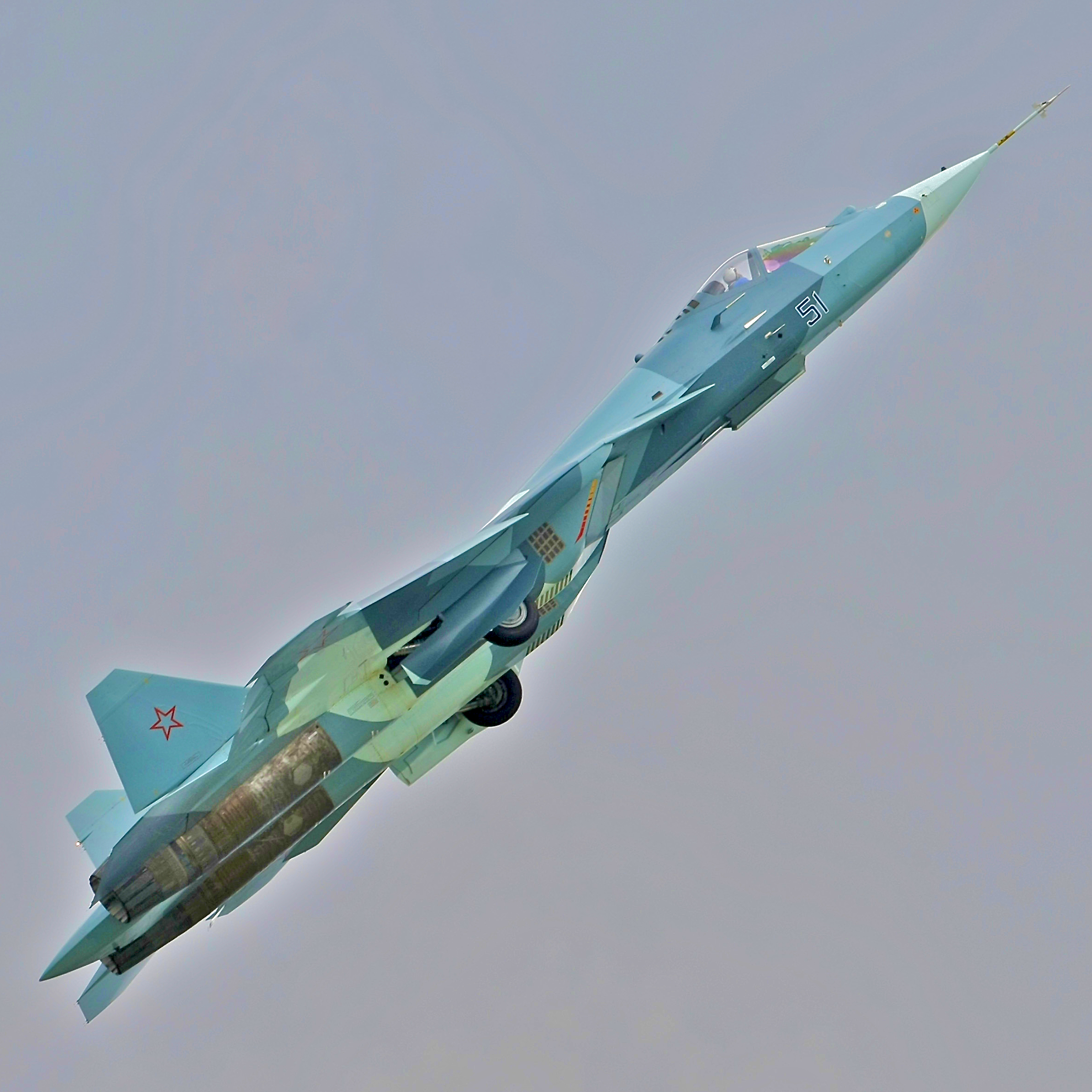 Sukhoi
T-50
prototype public demonstration [click to enlarge]. The shaping design
of
the T-50 presents no fundamental obstacles to its development into
a limited aspect coverage Very Low Observable design
(KnAAPO).
|
||||||||||||||||||||||||||||||||||||||||||||||||||||||||||||||||||||||||||||||||||||||||||||||||||||||||||||||||||||||||||||||||||||||||||||||||||||||||||||||||||||||||||||||||||||||||||||||||||||||
|
||||||||||||||||||||||||||||||||||||||||||||||||||||||||||||||||||||||||||||||||||||||||||||||||||||||||||||||||||||||||||||||||||||||||||||||||||||||||||||||||||||||||||||||||||||||||||||||||||||||
Index |
||||||||||||||||||||||||||||||||||||||||||||||||||||||||||||||||||||||||||||||||||||||||||||||||||||||||||||||||||||||||||||||||||||||||||||||||||||||||||||||||||||||||||||||||||||||||||||||||||||||
|
||||||||||||||||||||||||||||||||||||||||||||||||||||||||||||||||||||||||||||||||||||||||||||||||||||||||||||||||||||||||||||||||||||||||||||||||||||||||||||||||||||||||||||||||||||||||||||||||||||||
IntroductionThe Russian Sukhoi/KnAAPO T-50/I-21/Article 701 PAK-FA (Перспективный Авиационный Комплекс Фронтовой Авиации) was the first manned combat aircraft design intended to possess low observable capabilities in the radar bands to be developed and publicly flown by a nation other than the United States, the first public flight shown in early 20101. This paper extends earlier research focussed on the design of the T-50, and the Chengdu J-20, to provide a more accurate and quantitative preliminary assessment of the specular Radar Cross Section [RCS] of the T-50 design2,3. A full and comprehensive assessment of the RCS of any Low Observable [LO / -10 to -30 dBSM, Refer Table A.1] or Very Low Observable [VLO / -30 to -40 dBSM, Refer Table A.1] aircraft design is a non-trivial task, as careful consideration needs to be given to all major and minor RCS contributors in the design, of which there can be a large number in a complex design such as a combat aircraft. If such an assessment is to be genuinely useful, it must consider the vehicle's RCS from a range of different angular aspects encompassing azimuthal sectors and also elevation or depression angles characteristic of the surface and airborne threat systems the LO/VLO design is intended to defeat [Refer Figures A.3 and A.4]. The assessment of RCS must always be performed at the operating wavelengths typical of the surface and airborne threat systems the LO/VLO design is intended to defeat [Refer Table A.2]. Definitions of these and other terms employed in this document are summarised in Annex C. Reference data for RCS scales, radio-frequency bands, engagement geometries are summarised in Annex A. A summary of representative threat systems is available in Annex A, in an earlier publication3. The T-50 was developed specifically to compete against the F-22 Raptor in traditional Beyond Visual Range (BVR) and Within Visual Range (WVR) air combat. As a result, the T-50 shares all of the cardinal “fifth generation” attributes until now unique to the F-22 - stealth, supersonic cruise, thrust vectoring, highly integrated avionics and a powerful suite of active and passive sensors. The PAK-FA therefore firmly qualifies as a “fifth generation” design. In addition, it has two further attributes not introduced in the F-22 design. The first is “extreme plus agility”2, resulting from advanced aerodynamic design, exceptional thrust/weight ratio performance and three dimensional thrust vectoring integrated with an advanced digital flight control system. The second attribute is exceptional combat persistence, the result of an unusually large 25,000 lb internal fuel load. The former entailed some shaping compromises, at the expense of specular RCS performance. The basic shaping design observed on prototypes of the PAK-FA will deny it the critical all-aspect stealth performance of the F-22, critical in BVR air combat and deep penetration operations. Despite this, the extreme manoeuvrability/controllability design features of the PAK-FA, which result in extreme plus agility, result in the potential for the PAK-FA to become the most lethal and survivable fighter ever built for air combat engagements. The publicly displayed PAK-FA prototypes do not represent a production configuration of the aircraft, which is to employ a new engine design, and extensive VLO treatments which are not required on a prototype. This assessment, like the earlier assessment performed on the J-20 design, cannot be more than preliminary for a number of important reasons:
Proper airframe shaping, as stated in Denys Overholser's famous dictum, is a necessary and essential prerequisite for good LO or VLO performance. If shaping design is deficient, no amount of credible materials application and detail flare spot reduction can overcome the RCS contributions produced by the airframe shape, and genuine VLO performance will be therefore unattainable. While this is self-evident, it is often not well appreciated. If airframe shaping is credible, then careful and well considered application of Radar Absorbent Materials (RAM), Radar Absorbent Structures (RAS), radar absorbent coatings, aperture RCS reductions, and minor flare spot reduction techniques will yield a VLO design. Modelling of the shape related RCS contributions of any VLO design is of very high value, as it determines not only whether the aircraft can achieve credible VLO category performance, but also where the designers will be investing effort in RAS, RAM and coating application to achieve this effect. Moreover, it exposes the angular extents within which the aircraft has poor RCS performance, and thus provides a robust basis for development of tactics and technique to defeat the design. This paper will focus mostly on shape related RCS contributions, both due to the high value of knowing weaknesses in the design, but also due to the uncertainties inherent in estimating the performance of unknown technologies for RAS, RAM, coatings, aperture RCS reductions, and minor flare spot reduction. Where applicable, reasonable assumptions will be made as to the performance of absorbent material related RCS reduction measures. |
||||||||||||||||||||||||||||||||||||||||||||||||||||||||||||||||||||||||||||||||||||||||||||||||||||||||||||||||||||||||||||||||||||||||||||||||||||||||||||||||||||||||||||||||||||||||||||||||||||||
T-50 Prototype Very Low Observable Airframe Shaping Design Features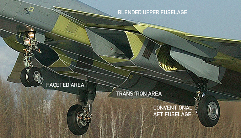 Figure 1. The lower fuselage of the prototype displays interesting incongruities. There is an abrupt transition between the carefully sculpted faceting of the inlet nacelles, and the smoothly curved aft engine nacelles and conventional aft fuselage. The faceting strategy is similar to the F-22 design rules, with singly or doubly curved transitions between planes (C. Kopp/Sukhoi image)2. An extensive qualitative analysis of RCS reduction shaping feature design in the T-50 aircraft was performed in 2010. That analysis yielded the following observations, cited here for convenience2:
The qualitative analysis yielded the conclusion that with proper application of materials technology, detail feature RCS reduction treatments, aperture structural mode RCS reduction measures, the T-50 had potential to yield viable VLO performance in the forward sector, and with a nozzle design similar to the F-22A, had potential for viable VLO performance in the aft sector. Performance in the beam sector and lower hemsiphere were identified as problematic. This conclusion was a result of several specific shaping features, specifically the lower fuselage tunnel design, and the absence of obtuse angle joins between the aft fuselage sides and wing / stabilator joins, and the obtuse join angles in the fuselage tunnel. Quantitative RCS modelling will demonstrate that these observations were valid. |
||||||||||||||||||||||||||||||||||||||||||||||||||||||||||||||||||||||||||||||||||||||||||||||||||||||||||||||||||||||||||||||||||||||||||||||||||||||||||||||||||||||||||||||||||||||||||||||||||||||
Radar
Cross Section Simulation Method / Simulator Design and Capabilities
|
||||||||||||||||||||||||||||||||||||||||||||||||||||||||||||||||||||||||||||||||||||||||||||||||||||||||||||||||||||||||||||||||||||||||||||||||||||||||||||||||||||||||||||||||||||||||||||||||||||||
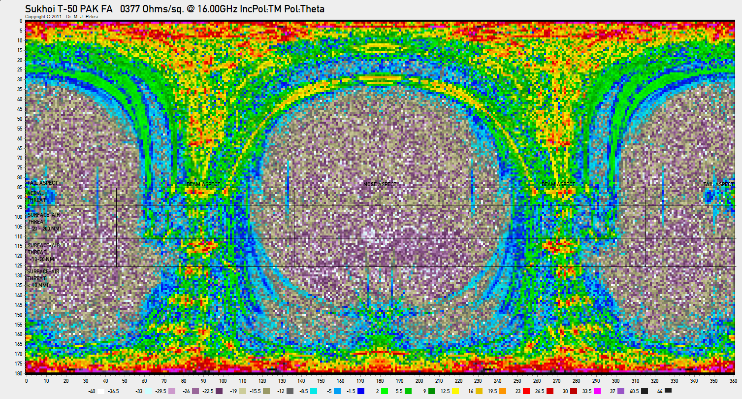
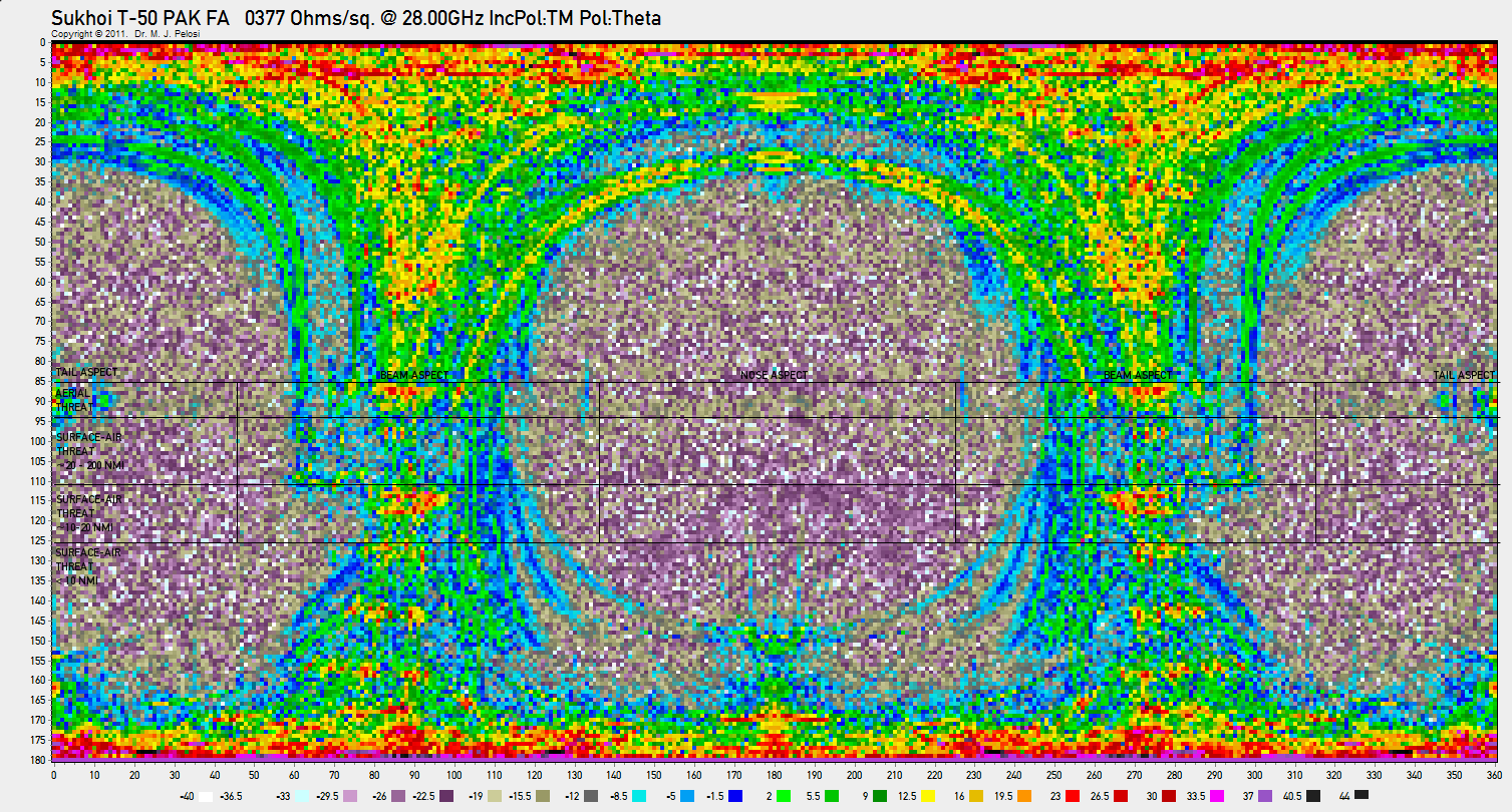
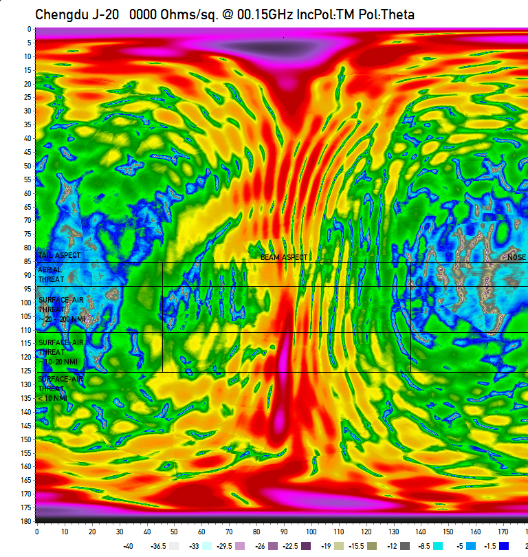
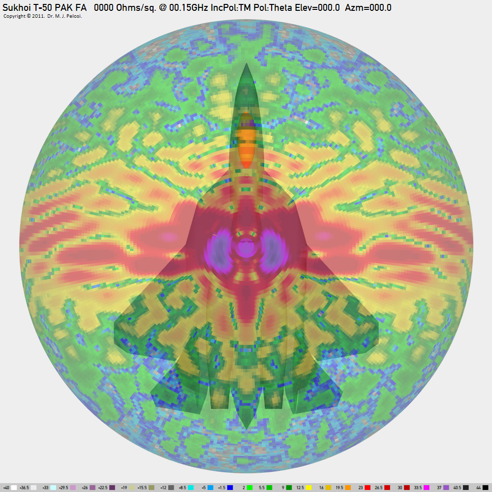
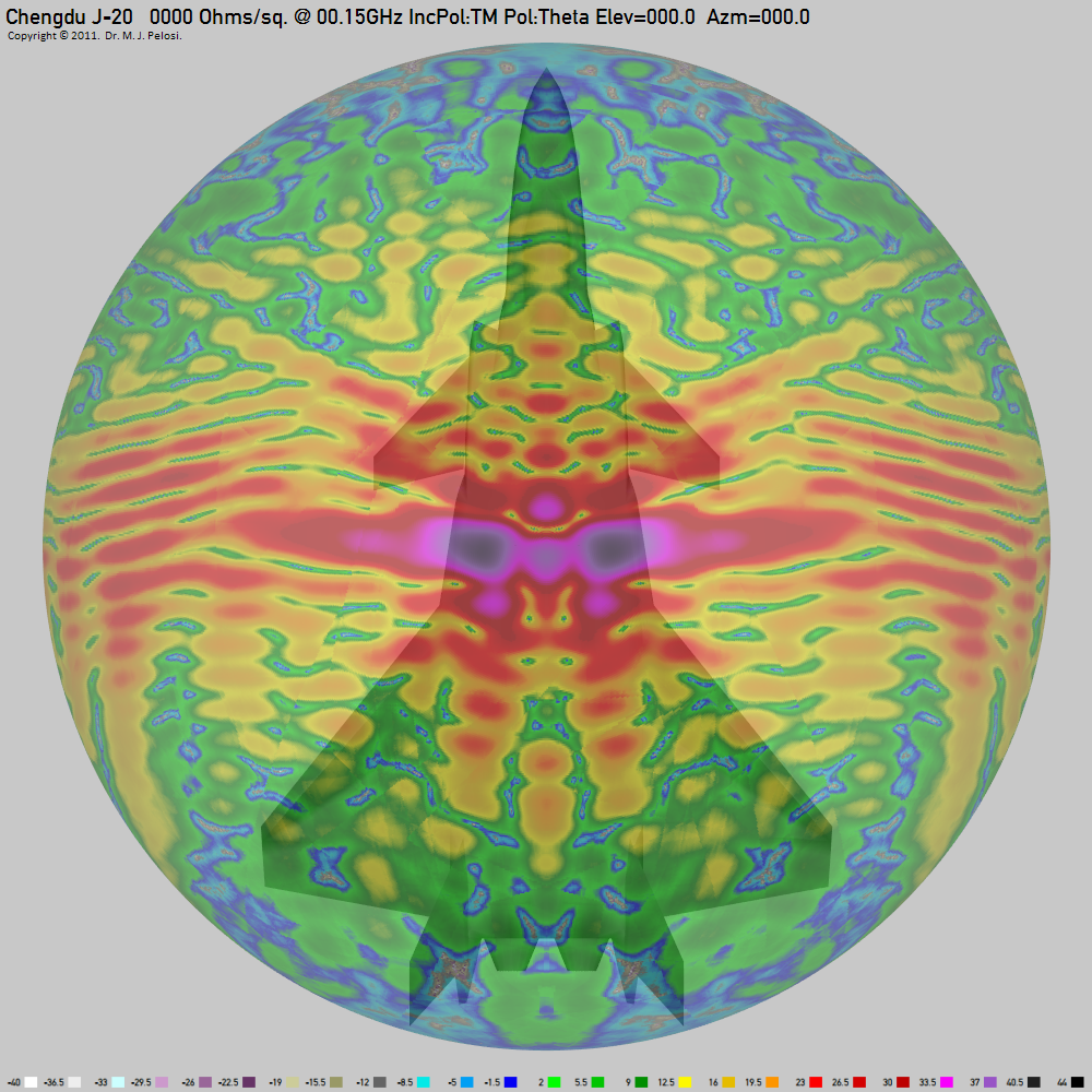
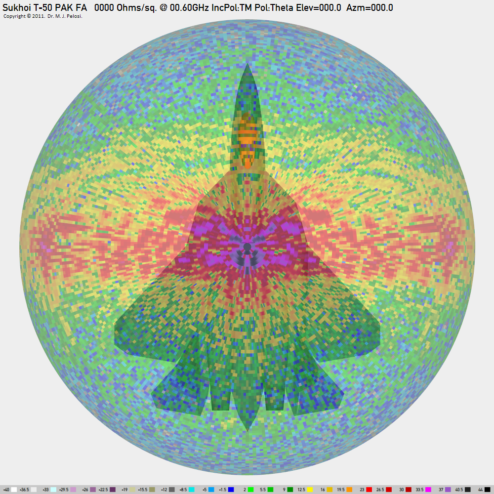
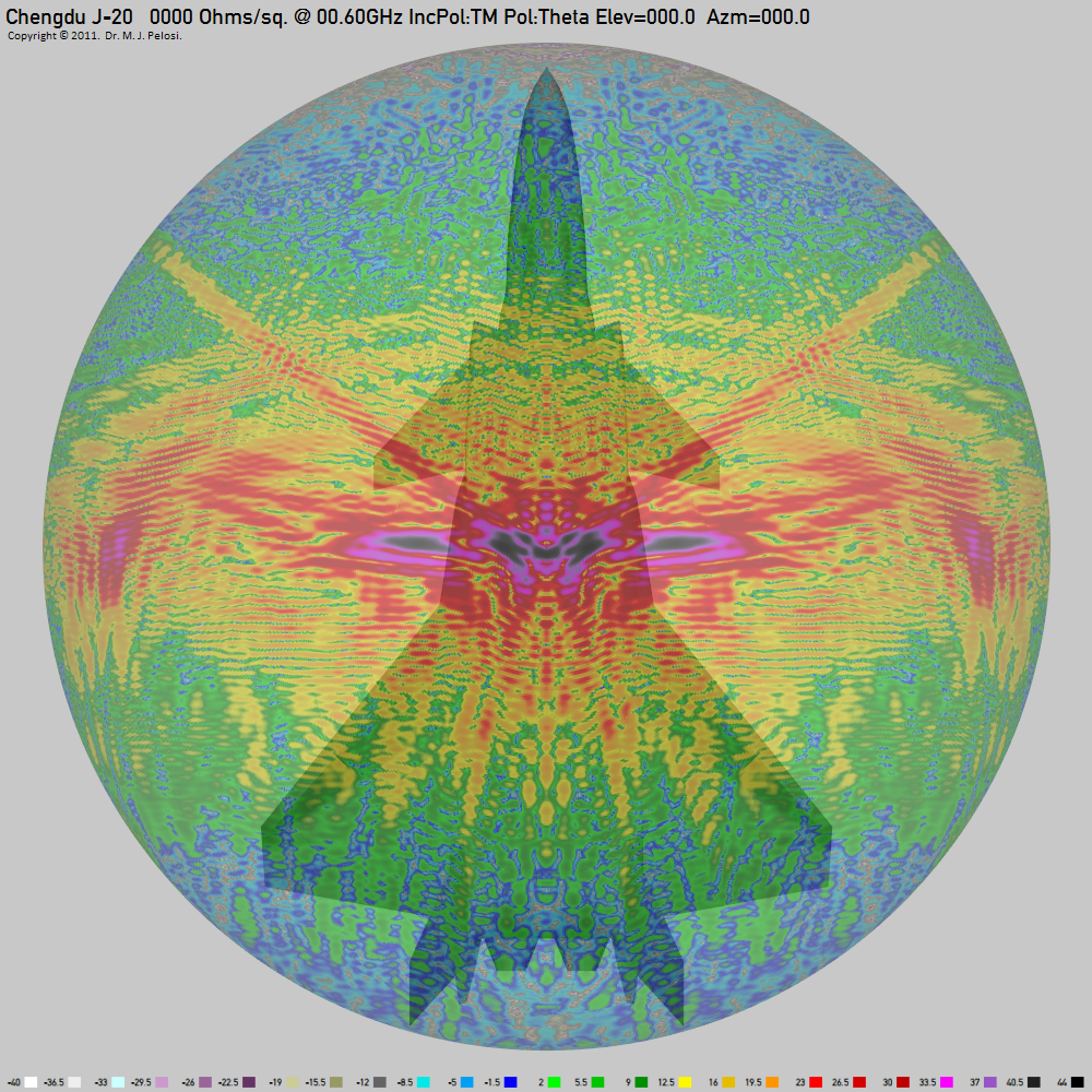
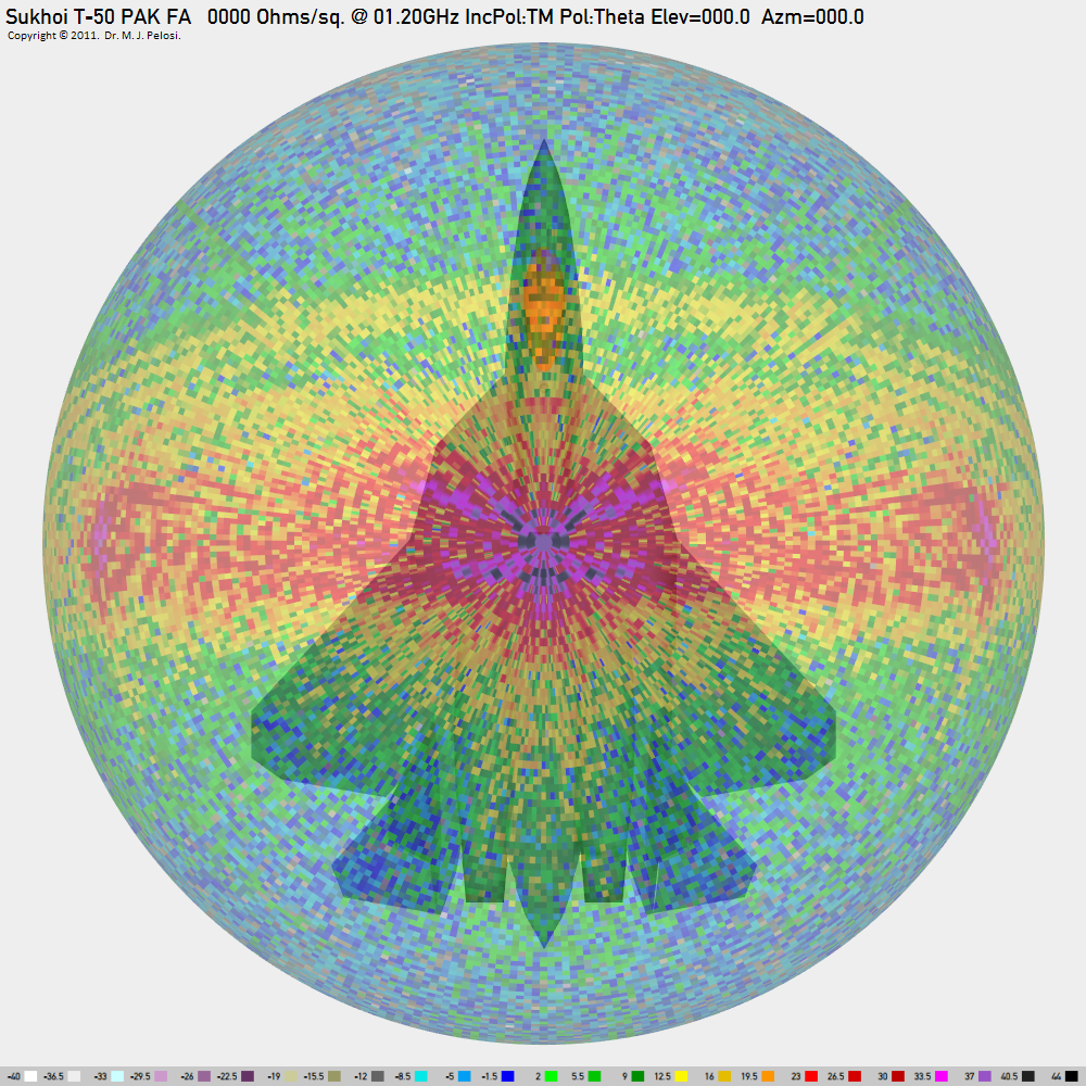
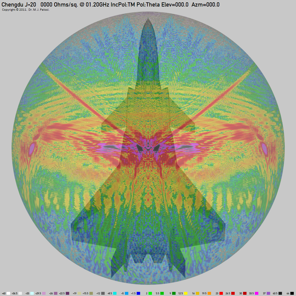
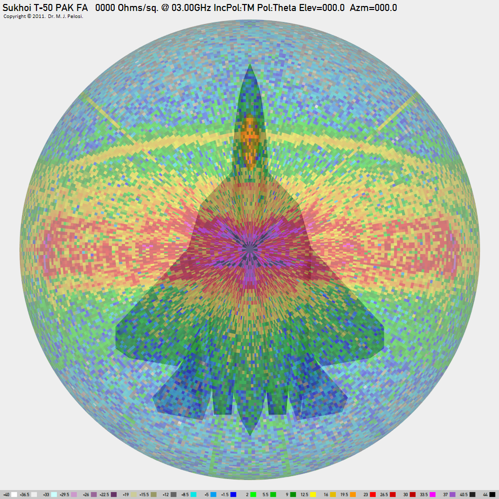
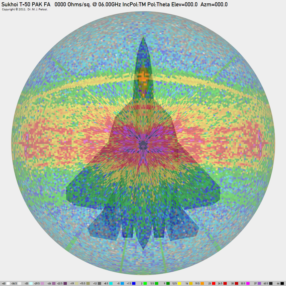
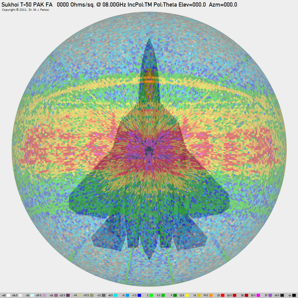
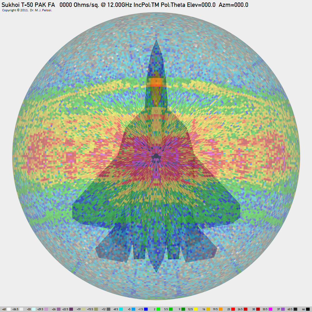
Specular Radar Cross Section Simulation ResultsSpecular RCS of the T-50 prototype was modelled for full spherical all-aspect coverage, for nine frequencies of interest. Frequencies were carefully chosen to match likely threat systems the T-50 would be intended to defeat in an operational environment. These chosen operating frequencies are: 150 MHz to defeat Chinese built VHF band Counter-VLO radars such as the CETC JY-27 Wide Mat, NRIET / CEIEC / CETC YLC-4, CETC YLC-8/8A and CPMIEC HK-JM28; 600 MHz to defeat UHF band radars such as those carried by the E-2C/D AEW&C system, or the widely exported Russian Kasta 2/2E and P-15/19 Flat Face / Squat Eye series; 1.2 GHz to defeat L-band surface based search, acquisition and GCI radars, and the Northrop-Grumman MESA AEW&C radar; 3.0 GHz to defeat widely used S-band acquisition radars, and the E-3 APY-1/APY-2 AWACS system; 6.0 GHz to defeat C-band Surface-Air-Missile engagement radars such as the MPQ-53/65 Patriot system; 8.0 GHz to defeat a range of X-band airborne fighter radars, Surface-Air-Missile engagement radars such as the 30N6E Flap Lid / Tomb Stone, and 92N6E Grave Stone, and a range of Western and Russian Surface-Air-Missile seekers; 12.0 GHz to defeat a range of X-band airborne fighter radars, Surface-Air-Missile engagement radars, and Surface-Air-Missile and Air-Air-Missile seekers; 16.0 GHz to defeat a range of Ku-band airborne fighter radars, and Surface-Air-Missile engagement radars, and Surface-Air-Missile and Air-Air-Missile seekers; 28.0 GHz to defeat a range of K-band missile seekers, and Surface-Air-Missile engagement radars; RCS simulation results are presented in PCSR and PCPR formats. The latter includes rulers to show the most important elevation/depression angle rings/zones, and the four azimuthal quadrants. Analysis of Shape Related Specular Radar Cross SectionThe results of the physical optics simulation modelling of specular RCS for the T-50 shape, using an idealised PEC skin for all external surfaces, are displayed in Tables 1 and 2, for a vertically polarised E component. Results have been plotted in PCSR format for nine different aspects, and nine different frequencies. PCPR format plots have been produced for nine different frequencies.
The PO modelling has validated all observations in the earlier qualitative analysis. Behaviour in the nose aspect angular sector, defined as ±45° in azimuth left and right of the nose, and between +5° in elevation, and -36° in depression, is mostly good across all bands simulated. This reflects attention paid to forward fuselage and inlet shaping and alignment, and presents no fundamental obstacles to attaining VLO performance in the nose aspect angular sector. No scattering sources introducing significant specular RCS contributions were observed at any of the modelled frequencies, although sidelobes from beam aspect scatterers begin to degrade the angular extent at UHF and VHF bands. Behaviour in the tail aspect angular sector, defined as ±45° in azimuth left and right of the tail, and between +5° in elevation, and -36° in depression, is clearly dominated by the scattering behaviour of the pair of axisymmetric nozzles, which has major specular, cavity and diffractive scattering contributions. The behaviour of such nozzles is well detailed in earlier work covering the F-35 JSF and J-20 nozzles5. Importantly, the T-50 prototypes employ an interim AL-41F1 powerplant, and associated three dimensional thrust vectoring nozzle developed for the conventional Su-27M2/Su-35S Flanker. Integration of this powerplant and nozzle introduces sub-optimal aft fuselage join geometry, and suboptimal axi-symmetric nozzles. To date there have been no definitive disclosures on the intended integration of the production powerplant, and its intended nozzle design. The aft fuselage geometry does not preclude the integration of a faceted VLO nozzle similar in concept to the F-22 design. Therefore, tail aspect angular sector specular RCS for production T-50 aircraft might be much superior to the prototypes, and competitive against the F-22. This is important from the perspective of technological strategy, as the T-50, like the J-20, has the evolutionary potential for robust VLO performance in the tail aspect angular sector, unlike the F-35 JSF, which is constrained by commonality to an axi-symmetric nozzle. The RCS of the untreated axi-symmetric nozzles observed on T-50 prototypes would be typically determined by the projected area of the aperture for a given aspect, and instantaneous position of the 3D TVC nozzle, and thus of the order of 1 m2 in the aft sector, and presenting significant contributions in the nose sector. The location of the major lobes produced by the nozzle will depend strongly on the instantaneous position. Axi-symmetric nozzle contributions are discussed in some detail in previous work5. Behaviour in the left and right beam aspect angular sectors, defined as ±45° in azimuth left and right of the beam, and between +5° in elevation, and -36° in depression, presents an interesting case study. The grouping of primary scattering lobes in the beam aspect is quite unique in the T-50 design. The F-22 presents as a “two lobe” design and the J-20 presents as “three lobe” design, contrasting distinctly against the defacto “single lobe” design of the F-35, where complex lower fuselage convex and concave double curvatures effectively merge multiple lesser lobes into a single wide angle specular scatterer. The latter is the worst possible strategy for managing beam aspect lobes as it minimises the variation of specular return peak magnitude with elevation/depression angle. The T-50 presents as a “six lobe” design, with specular slab reflectors and corner reflectors aligned to concentrate beam aspect backscatter into one normal ventral lobe, and five staggered lobes pointing sideways at different elevation/depression angles. This is depicted in Figures 3 and 4. The strongest peak is in the “C” lobe, centred at a depression angle of about -25° in depression. 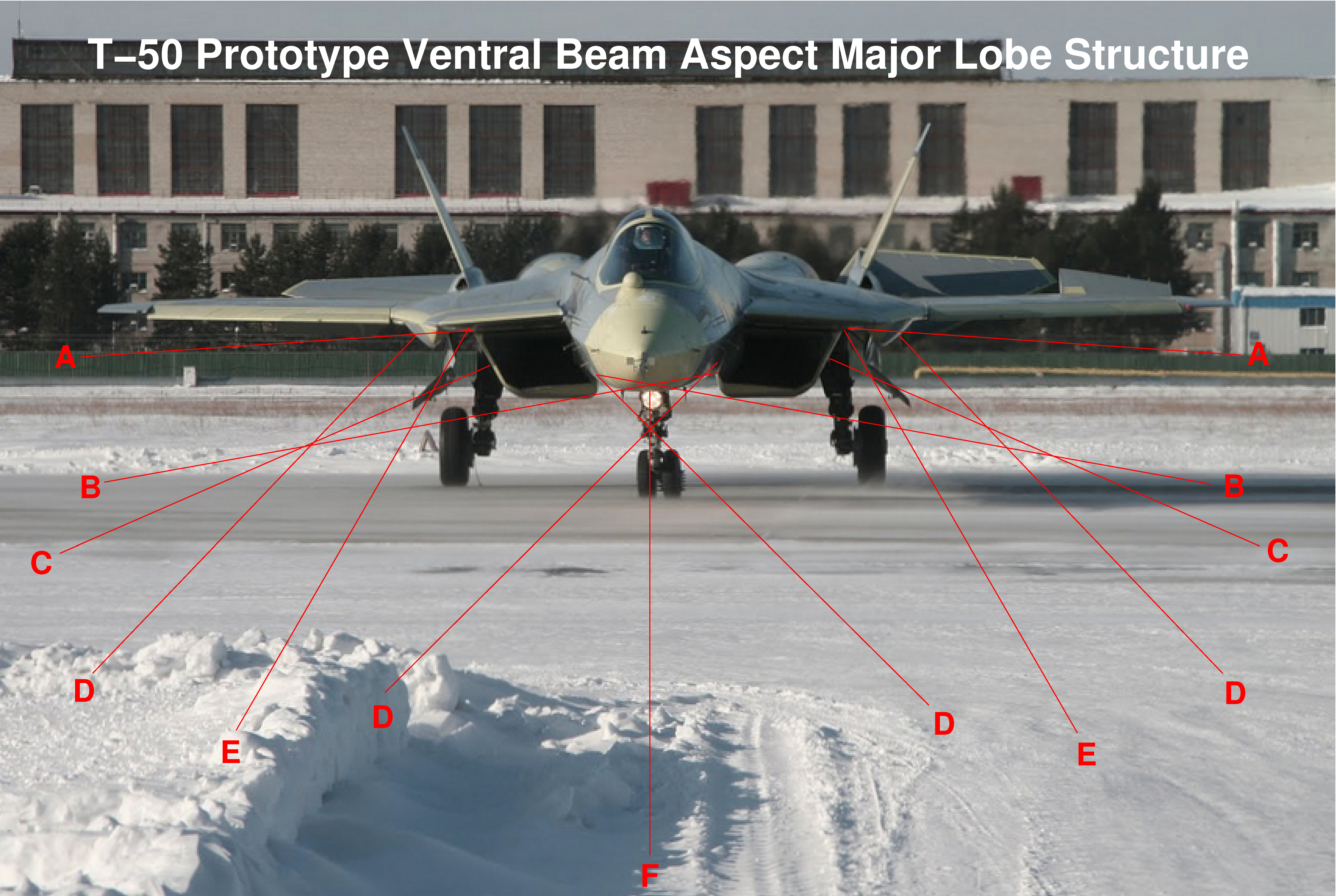 Figure 3. The T-50 has five major lobes in the left and right beam aspect angular sectors, for convenience labelled A through E, with the flat lower fuselage mainlobe labelled F (KnAAPO image). 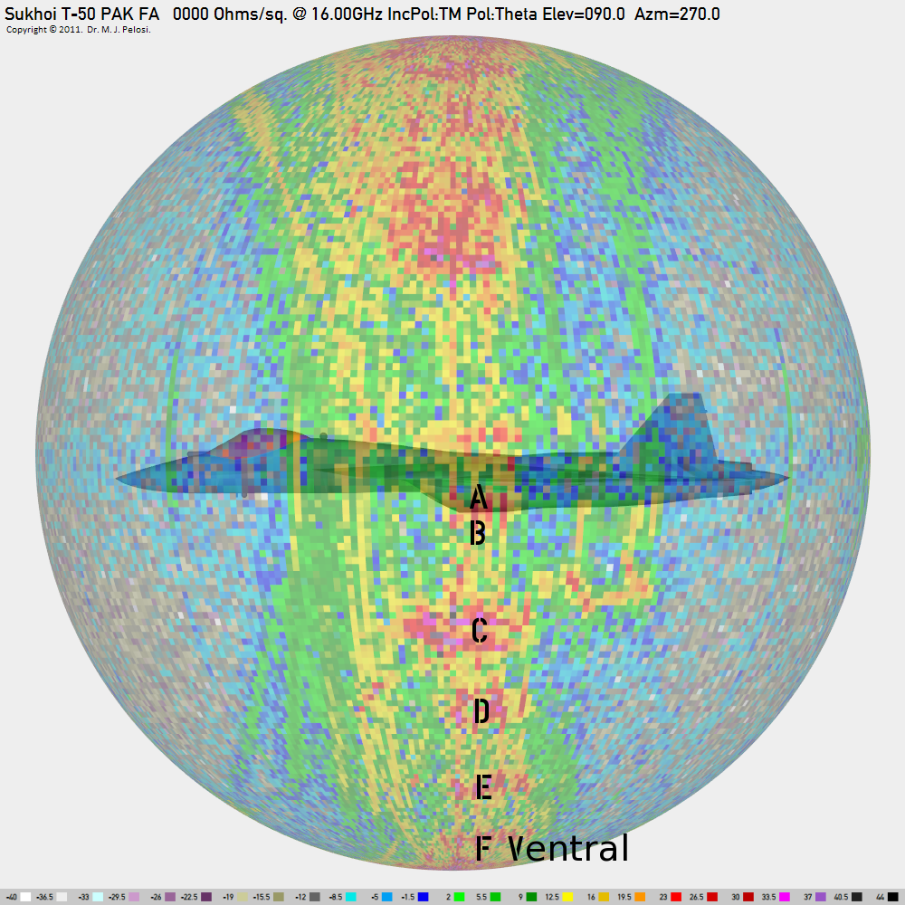 Figure 4. Mapping of the five major lobes in the left and right beam aspect angular sectors at 16 GHz (KnAAPO image). 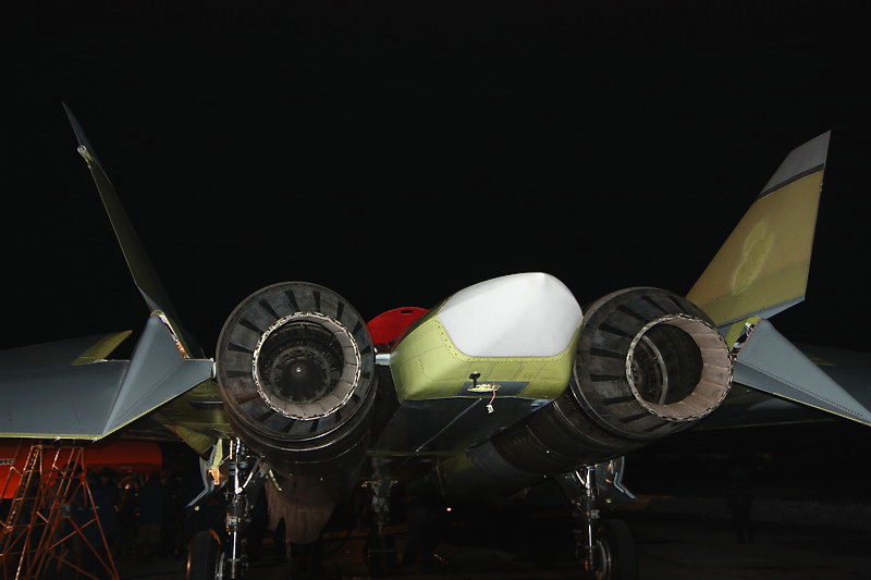 Figure 5. The T-50 from behind,
showing the corner joins in the inlet tunnel, and fuselage sides
(KnAAPO image).
The association of the beam aspect mainlobes can be readily established from specific shaping features in the design.
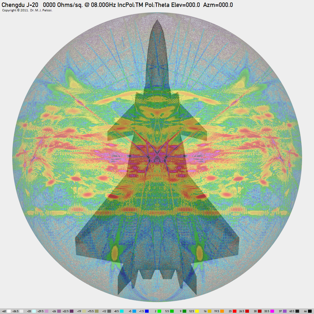
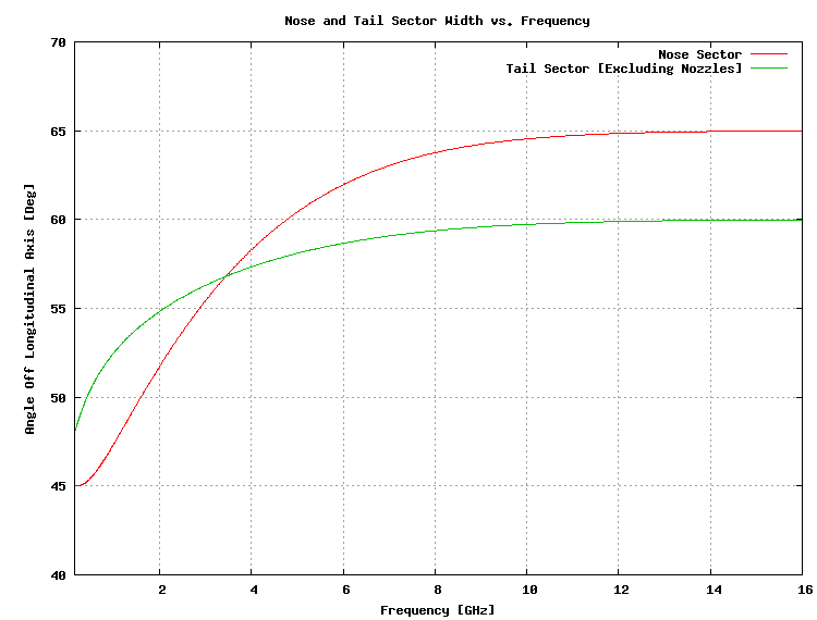 Figure 6. Frequency dependency of the angle off the longitudinal axis at which beam aspect lobe magnitude exceeds +2 dBSM, for depression angles of less than -25°. The horizontal angular width of the nose and tail aspect VLO range can be estimated by doubling the plotted value for the frequency of interest. In summary, beam aspect specular RCS is dominated by the scattering behaviour of the almost flat slab sides, canted vertical tail surfaces, and specular return from the nozzles. This could be described as classical “bowtie” lobing behaviour, with the caveat that if the axisymmetric nozzle is retained in production aircraft, the detrimental impact of the nozzles will yield undesirable “pacman” lobing behaviour, not unlike the F-35 aircraft. Some comparisons with other aircraft types are warranted, given the dominant effect of specular scattering mechanisms in beam aspect RCS, and the importance of beam aspect RCS in defence penetration, and air combat situations where fighter threats may present from any aspect. The shaping of the T-50 is inferior to that of the F-22 Raptor. This is mostly a byproduct of the significantly more complex shaping of the lower fuselage area, the use of a tunnel between the engine nacelles, and the aft fuselage join between the aft engine nacelles, and fuselage at the wing and stabilator roots. The single narrow specular mainlobe produced by the careful shaping and fuselage joining of the F-22 presents a much smaller visible angular extent compared to the T-50. The J-20, which largely emulates the advantages of the F-22 Raptor shaping configuration, is also superior to the T-50, but by a less distinct margin than the F-22 Raptor. Annex E presents a direct comparison of the specular RCS plots for both types. The J-20 performs better at higher frequencies, where the greater length of linear shaping features is better able to control mainlobe width. The F-35 JSF exhibits similar, but in some respects more severe beam aspect specular RCS behaviour than the T-50. This is a direct consequence of the use of multiple complex double curvature convex and concave shaping features in its lower fuselage design, and lower wing root area, and a much shorter fuselage. The ventral shaping features were introduced in the SDD aircraft and were not part of the X-35 demonstrator design. Another unfortunate feature of F-35 shaping is the depression angle of the slab sides of the engine inlets, which is shallower than the F-22 and J-20 designs, and similar to the T-50, as a result of which the associated mainlobe peaks at a lesser depression angle, in turn degrading performance against long range surface based threats. The conclusion which can be drawn from forensic analysis of the T-50 PAK-FA specular RCS modelling for a conductive surface is that its specular RCS performance will satisfy the Very Low Observable requirement that strong specular returns are absent in the nose sector angular domain. In this angular and frequency domain, i.e forward sector and S-band and above, the actual RCS performance of the design will be dominated by edge alignment to control diffracting edge mainlobe directions, and applied RAM and RAS, i.e. materials technology. |
||||||||||||||||||||||||||||||||||||||||||||||||||||||||||||||||||||||||||||||||||||||||||||||||||||||||||||||||||||||||||||||||||||||||||||||||||||||||||||||||||||||||||||||||||||||||||||||||||||||
Analysis of
Specular RCS with a RAM Coating
|
||||||||||||||||||||||||||||||||||||||||||||||||||||||||||||||||||||||||||||||||||||||||||||||||||||||||||||||||||||||||||||||||||||||||||||||||||||||||||||||||||||||||||||||||||||||||||||||||||||||
![Sukhoi-T-50-PAK-FA.mdb-00.15GHz-Rs0000-IncPol-TM-Pol-Theta-[E=180.0-A=180.0]](Rus-VLO/Sukhoi-T-50-PAK-FA.mdb-00.15GHz-Rs0000-IncPol-TM-Pol-Theta-%5BE=180.0-A=180.0%5D.png "Sukhoi-T-50-PAK-FA.mdb-00.15GHz-Rs0000-IncPol-TM-Pol-Theta-[E=180.0-A=180.0]")
![Sukhoi-T-50-PAK-FA.mdb-01.20GHz-Rs0000-IncPol-TM-Pol-Theta-[E=180.0-A=180.0]](Rus-VLO/Sukhoi-T-50-PAK-FA.mdb-01.20GHz-Rs0000-IncPol-TM-Pol-Theta-%5BE=180.0-A=180.0%5D.png "Sukhoi-T-50-PAK-FA.mdb-01.20GHz-Rs0000-IncPol-TM-Pol-Theta-[E=180.0-A=180.0]")
![Sukhoi-T-50-PAK-FA.mdb-03.00GHz-Rs0000-IncPol-TM-Pol-Theta-[E=180.0-A=180.0]](Rus-VLO/Sukhoi-T-50-PAK-FA.mdb-03.00GHz-Rs0000-IncPol-TM-Pol-Theta-%5BE=180.0-A=180.0%5D.png "Sukhoi-T-50-PAK-FA.mdb-03.00GHz-Rs0000-IncPol-TM-Pol-Theta-[E=180.0-A=180.0]")
![Sukhoi-T-50-PAK-FA.mdb-06.00GHz-Rs0000-IncPol-TM-Pol-Theta-[E=180.0-A=180.0]](Rus-VLO/Sukhoi-T-50-PAK-FA.mdb-06.00GHz-Rs0000-IncPol-TM-Pol-Theta-%5BE=180.0-A=180.0%5D.png "Sukhoi-T-50-PAK-FA.mdb-06.00GHz-Rs0000-IncPol-TM-Pol-Theta-[E=180.0-A=180.0]")
![Sukhoi-T-50-PAK-FA.mdb-08.00GHz-Rs0000-IncPol-TM-Pol-Theta-[E=180.0-A=180.0]](Rus-VLO/Sukhoi-T-50-PAK-FA.mdb-08.00GHz-Rs0000-IncPol-TM-Pol-Theta-%5BE=180.0-A=180.0%5D.png "Sukhoi-T-50-PAK-FA.mdb-08.00GHz-Rs0000-IncPol-TM-Pol-Theta-[E=180.0-A=180.0]")
![Sukhoi-T-50-PAK-FA.mdb-12.00GHz-Rs0000-IncPol-TM-Pol-Theta-[E=180.0-A=180.0]](Rus-VLO/Sukhoi-T-50-PAK-FA.mdb-12.00GHz-Rs0000-IncPol-TM-Pol-Theta-%5BE=180.0-A=180.0%5D.png "Sukhoi-T-50-PAK-FA.mdb-12.00GHz-Rs0000-IncPol-TM-Pol-Theta-[E=180.0-A=180.0]")
![Sukhoi-T-50-PAK-FA.mdb-16.00GHz-Rs0000-IncPol-TM-Pol-Theta-[E=180.0-A=180.0]](Rus-VLO/Sukhoi-T-50-PAK-FA.mdb-16.00GHz-Rs0000-IncPol-TM-Pol-Theta-%5BE=180.0-A=180.0%5D.png "Sukhoi-T-50-PAK-FA.mdb-16.00GHz-Rs0000-IncPol-TM-Pol-Theta-[E=180.0-A=180.0]")
![Sukhoi-T-50-PAK-FA.mdb-28.00GHz-Rs0000-IncPol-TM-Pol-Theta-[E=180.0-A=180.0]](Rus-VLO/Sukhoi-T-50-PAK-FA.mdb-28.00GHz-Rs0000-IncPol-TM-Pol-Theta-%5BE=180.0-A=180.0%5D.png "Sukhoi-T-50-PAK-FA.mdb-28.00GHz-Rs0000-IncPol-TM-Pol-Theta-[E=180.0-A=180.0]")
![Sukhoi-T-50-PAK-FA.mdb-00.15GHz-Rs0000-IncPol-TM-Pol-Theta-[E=090.0-A=180.0]](Rus-VLO/Sukhoi-T-50-PAK-FA.mdb-00.15GHz-Rs0000-IncPol-TM-Pol-Theta-%5BE=090.0-A=180.0%5D.png "Sukhoi-T-50-PAK-FA.mdb-00.15GHz-Rs0000-IncPol-TM-Pol-Theta-[E=090.0-A=180.0]")
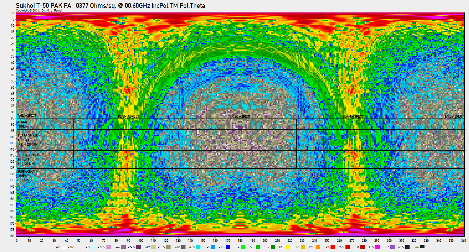
![Sukhoi-T-50-PAK-FA.mdb-00.60GHz-Rs0000-IncPol-TM-Pol-Theta-[E=090.0-A=180.0]](Rus-VLO/Sukhoi-T-50-PAK-FA.mdb-00.60GHz-Rs0000-IncPol-TM-Pol-Theta-%5BE=090.0-A=180.0%5D.png "Sukhoi-T-50-PAK-FA.mdb-00.60GHz-Rs0000-IncPol-TM-Pol-Theta-[E=090.0-A=180.0]")
![Sukhoi-T-50-PAK-FA.mdb-01.20GHz-Rs0000-IncPol-TM-Pol-Theta-[E=090.0-A=180.0]](Rus-VLO/Sukhoi-T-50-PAK-FA.mdb-01.20GHz-Rs0000-IncPol-TM-Pol-Theta-%5BE=090.0-A=180.0%5D.png "Sukhoi-T-50-PAK-FA.mdb-01.20GHz-Rs0000-IncPol-TM-Pol-Theta-[E=090.0-A=180.0]")
![Sukhoi-T-50-PAK-FA.mdb-03.00GHz-Rs0000-IncPol-TM-Pol-Theta-[E=090.0-A=180.0]](Rus-VLO/Sukhoi-T-50-PAK-FA.mdb-03.00GHz-Rs0000-IncPol-TM-Pol-Theta-%5BE=090.0-A=180.0%5D.png "Sukhoi-T-50-PAK-FA.mdb-03.00GHz-Rs0000-IncPol-TM-Pol-Theta-[E=090.0-A=180.0]")
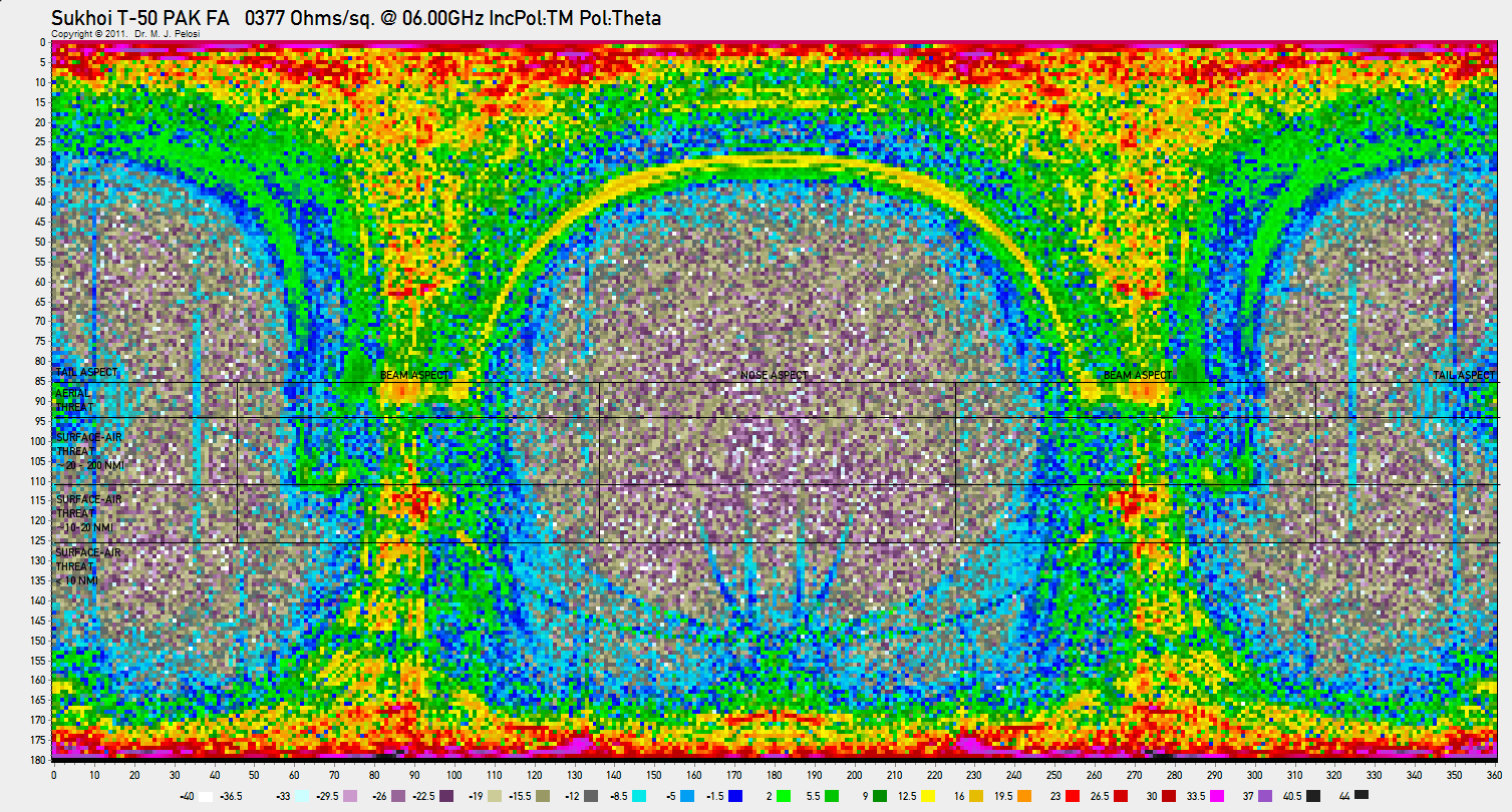
![Sukhoi-T-50-PAK-FA.mdb-06.00GHz-Rs0000-IncPol-TM-Pol-Theta-[E=090.0-A=180.0]](Rus-VLO/Sukhoi-T-50-PAK-FA.mdb-06.00GHz-Rs0000-IncPol-TM-Pol-Theta-%5BE=090.0-A=180.0%5D.png "Sukhoi-T-50-PAK-FA.mdb-06.00GHz-Rs0000-IncPol-TM-Pol-Theta-[E=090.0-A=180.0]")
![Sukhoi-T-50-PAK-FA.mdb-08.00GHz-Rs0000-IncPol-TM-Pol-Theta-[E=090.0-A=180.0]](Rus-VLO/Sukhoi-T-50-PAK-FA.mdb-08.00GHz-Rs0000-IncPol-TM-Pol-Theta-%5BE=090.0-A=180.0%5D.png "Sukhoi-T-50-PAK-FA.mdb-08.00GHz-Rs0000-IncPol-TM-Pol-Theta-[E=090.0-A=180.0]")
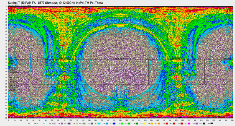
![Sukhoi-T-50-PAK-FA.mdb-12.00GHz-Rs0000-IncPol-TM-Pol-Theta-[E=090.0-A=180.0]](Rus-VLO/Sukhoi-T-50-PAK-FA.mdb-12.00GHz-Rs0000-IncPol-TM-Pol-Theta-%5BE=090.0-A=180.0%5D.png "Sukhoi-T-50-PAK-FA.mdb-12.00GHz-Rs0000-IncPol-TM-Pol-Theta-[E=090.0-A=180.0]")
![Sukhoi-T-50-PAK-FA.mdb-16.00GHz-Rs0000-IncPol-TM-Pol-Theta-[E=090.0-A=180.0]](Rus-VLO/Sukhoi-T-50-PAK-FA.mdb-16.00GHz-Rs0000-IncPol-TM-Pol-Theta-%5BE=090.0-A=180.0%5D.png "Sukhoi-T-50-PAK-FA.mdb-16.00GHz-Rs0000-IncPol-TM-Pol-Theta-[E=090.0-A=180.0]")
![Sukhoi-T-50-PAK-FA.mdb-28.00GHz-Rs0000-IncPol-TM-Pol-Theta-[E=090.0-A=180.0]](Rus-VLO/Sukhoi-T-50-PAK-FA.mdb-28.00GHz-Rs0000-IncPol-TM-Pol-Theta-%5BE=090.0-A=180.0%5D.png "Sukhoi-T-50-PAK-FA.mdb-28.00GHz-Rs0000-IncPol-TM-Pol-Theta-[E=090.0-A=180.0]")
![Sukhoi-T-50-PAK-FA.mdb-00.15GHz-Rs0000-IncPol-TM-Pol-Theta-[E=090.0-A=000.0]](Rus-VLO/Sukhoi-T-50-PAK-FA.mdb-00.15GHz-Rs0000-IncPol-TM-Pol-Theta-%5BE=090.0-A=000.0%5D.png "Sukhoi-T-50-PAK-FA.mdb-00.15GHz-Rs0000-IncPol-TM-Pol-Theta-[E=090.0-A=000.0]")
![Sukhoi-T-50-PAK-FA.mdb-00.60GHz-Rs0000-IncPol-TM-Pol-Theta-[E=090.0-A=000.0]](Rus-VLO/Sukhoi-T-50-PAK-FA.mdb-00.60GHz-Rs0000-IncPol-TM-Pol-Theta-%5BE=090.0-A=000.0%5D.png "Sukhoi-T-50-PAK-FA.mdb-00.60GHz-Rs0000-IncPol-TM-Pol-Theta-[E=090.0-A=000.0]")
![Sukhoi-T-50-PAK-FA.mdb-01.20GHz-Rs0000-IncPol-TM-Pol-Theta-[E=090.0-A=000.0]](Rus-VLO/Sukhoi-T-50-PAK-FA.mdb-01.20GHz-Rs0000-IncPol-TM-Pol-Theta-%5BE=090.0-A=000.0%5D.png "Sukhoi-T-50-PAK-FA.mdb-01.20GHz-Rs0000-IncPol-TM-Pol-Theta-[E=090.0-A=000.0]")
![Sukhoi-T-50-PAK-FA.mdb-03.00GHz-Rs0000-IncPol-TM-Pol-Theta-[E=090.0-A=000.0]](Rus-VLO/Sukhoi-T-50-PAK-FA.mdb-03.00GHz-Rs0000-IncPol-TM-Pol-Theta-%5BE=090.0-A=000.0%5D.png "Sukhoi-T-50-PAK-FA.mdb-03.00GHz-Rs0000-IncPol-TM-Pol-Theta-[E=090.0-A=000.0]")
![Sukhoi-T-50-PAK-FA.mdb-06.00GHz-Rs0000-IncPol-TM-Pol-Theta-[E=090.0-A=000.0]](Rus-VLO/Sukhoi-T-50-PAK-FA.mdb-06.00GHz-Rs0000-IncPol-TM-Pol-Theta-%5BE=090.0-A=000.0%5D.png "Sukhoi-T-50-PAK-FA.mdb-06.00GHz-Rs0000-IncPol-TM-Pol-Theta-[E=090.0-A=000.0]")
![Sukhoi-T-50-PAK-FA.mdb-08.00GHz-Rs0000-IncPol-TM-Pol-Theta-[E=090.0-A=000.0]](Rus-VLO/Sukhoi-T-50-PAK-FA.mdb-08.00GHz-Rs0000-IncPol-TM-Pol-Theta-%5BE=090.0-A=000.0%5D.png "Sukhoi-T-50-PAK-FA.mdb-08.00GHz-Rs0000-IncPol-TM-Pol-Theta-[E=090.0-A=000.0]")
![Sukhoi-T-50-PAK-FA.mdb-12.00GHz-Rs0000-IncPol-TM-Pol-Theta-[E=090.0-A=000.0]](Rus-VLO/Sukhoi-T-50-PAK-FA.mdb-12.00GHz-Rs0000-IncPol-TM-Pol-Theta-%5BE=090.0-A=000.0%5D.png "Sukhoi-T-50-PAK-FA.mdb-12.00GHz-Rs0000-IncPol-TM-Pol-Theta-[E=090.0-A=000.0]")
![Sukhoi-T-50-PAK-FA.mdb-16.00GHz-Rs0000-IncPol-TM-Pol-Theta-[E=090.0-A=000.0]](Rus-VLO/Sukhoi-T-50-PAK-FA.mdb-16.00GHz-Rs0000-IncPol-TM-Pol-Theta-%5BE=090.0-A=000.0%5D.png "Sukhoi-T-50-PAK-FA.mdb-16.00GHz-Rs0000-IncPol-TM-Pol-Theta-[E=090.0-A=000.0]")
![Sukhoi-T-50-PAK-FA.mdb-28.00GHz-Rs0000-IncPol-TM-Pol-Theta-[E=090.0-A=000.0]](Rus-VLO/Sukhoi-T-50-PAK-FA.mdb-28.00GHz-Rs0000-IncPol-TM-Pol-Theta-%5BE=090.0-A=000.0%5D.png "Sukhoi-T-50-PAK-FA.mdb-28.00GHz-Rs0000-IncPol-TM-Pol-Theta-[E=090.0-A=000.0]")
![Sukhoi-T-50-PAK-FA.mdb-00.15GHz-Rs0000-IncPol-TM-Pol-Theta-[E=090.0-A=270.0]](Rus-VLO/Sukhoi-T-50-PAK-FA.mdb-00.15GHz-Rs0000-IncPol-TM-Pol-Theta-%5BE=090.0-A=270.0%5D.png "Sukhoi-T-50-PAK-FA.mdb-00.15GHz-Rs0000-IncPol-TM-Pol-Theta-[E=090.0-A=270.0]")
![Sukhoi-T-50-PAK-FA.mdb-00.60GHz-Rs0000-IncPol-TM-Pol-Theta-[E=090.0-A=270.0]](Rus-VLO/Sukhoi-T-50-PAK-FA.mdb-00.60GHz-Rs0000-IncPol-TM-Pol-Theta-%5BE=090.0-A=270.0%5D.png "Sukhoi-T-50-PAK-FA.mdb-00.60GHz-Rs0000-IncPol-TM-Pol-Theta-[E=090.0-A=270.0]")
![Sukhoi-T-50-PAK-FA.mdb-01.20GHz-Rs0000-IncPol-TM-Pol-Theta-[E=090.0-A=270.0]](Rus-VLO/Sukhoi-T-50-PAK-FA.mdb-01.20GHz-Rs0000-IncPol-TM-Pol-Theta-%5BE=090.0-A=270.0%5D.png "Sukhoi-T-50-PAK-FA.mdb-01.20GHz-Rs0000-IncPol-TM-Pol-Theta-[E=090.0-A=270.0]")
![Sukhoi-T-50-PAK-FA.mdb-03.00GHz-Rs0000-IncPol-TM-Pol-Theta-[E=090.0-A=270.0]](Rus-VLO/Sukhoi-T-50-PAK-FA.mdb-03.00GHz-Rs0000-IncPol-TM-Pol-Theta-%5BE=090.0-A=270.0%5D.png "Sukhoi-T-50-PAK-FA.mdb-03.00GHz-Rs0000-IncPol-TM-Pol-Theta-[E=090.0-A=270.0]")
![Sukhoi-T-50-PAK-FA.mdb-06.00GHz-Rs0000-IncPol-TM-Pol-Theta-[E=090.0-A=270.0]](Rus-VLO/Sukhoi-T-50-PAK-FA.mdb-06.00GHz-Rs0000-IncPol-TM-Pol-Theta-%5BE=090.0-A=270.0%5D.png "Sukhoi-T-50-PAK-FA.mdb-06.00GHz-Rs0000-IncPol-TM-Pol-Theta-[E=090.0-A=270.0]")
![Sukhoi-T-50-PAK-FA.mdb-08.00GHz-Rs0000-IncPol-TM-Pol-Theta-[E=090.0-A=270.0]](Rus-VLO/Sukhoi-T-50-PAK-FA.mdb-08.00GHz-Rs0000-IncPol-TM-Pol-Theta-%5BE=090.0-A=270.0%5D.png "Sukhoi-T-50-PAK-FA.mdb-08.00GHz-Rs0000-IncPol-TM-Pol-Theta-[E=090.0-A=270.0]")
![Sukhoi-T-50-PAK-FA.mdb-12.00GHz-Rs0000-IncPol-TM-Pol-Theta-[E=090.0-A=270.0]](Rus-VLO/Sukhoi-T-50-PAK-FA.mdb-12.00GHz-Rs0000-IncPol-TM-Pol-Theta-%5BE=090.0-A=270.0%5D.png "Sukhoi-T-50-PAK-FA.mdb-12.00GHz-Rs0000-IncPol-TM-Pol-Theta-[E=090.0-A=270.0]")
![Sukhoi-T-50-PAK-FA.mdb-16.00GHz-Rs0000-IncPol-TM-Pol-Theta-[E=090.0-A=270.0]](Rus-VLO/Sukhoi-T-50-PAK-FA.mdb-16.00GHz-Rs0000-IncPol-TM-Pol-Theta-%5BE=090.0-A=270.0%5D.png "Sukhoi-T-50-PAK-FA.mdb-16.00GHz-Rs0000-IncPol-TM-Pol-Theta-[E=090.0-A=270.0]")
![Sukhoi-T-50-PAK-FA.mdb-28.00GHz-Rs0000-IncPol-TM-Pol-Theta-[E=090.0-A=270.0]](Rus-VLO/Sukhoi-T-50-PAK-FA.mdb-28.00GHz-Rs0000-IncPol-TM-Pol-Theta-%5BE=090.0-A=270.0%5D.png "Sukhoi-T-50-PAK-FA.mdb-28.00GHz-Rs0000-IncPol-TM-Pol-Theta-[E=090.0-A=270.0]")
![Sukhoi-T-50-PAK-FA.mdb-00.60GHz-Rs0000-IncPol-TM-Pol-Theta-[E=045.0-A=225.0]](Rus-VLO/Sukhoi-T-50-PAK-FA.mdb-00.60GHz-Rs0000-IncPol-TM-Pol-Theta-%5BE=045.0-A=225.0%5D.png "Sukhoi-T-50-PAK-FA.mdb-00.60GHz-Rs0000-IncPol-TM-Pol-Theta-[E=045.0-A=225.0]")
![Sukhoi-T-50-PAK-FA.mdb-01.20GHz-Rs0000-IncPol-TM-Pol-Theta-[E=045.0-A=225.0]](Rus-VLO/Sukhoi-T-50-PAK-FA.mdb-01.20GHz-Rs0000-IncPol-TM-Pol-Theta-%5BE=045.0-A=225.0%5D.png "Sukhoi-T-50-PAK-FA.mdb-01.20GHz-Rs0000-IncPol-TM-Pol-Theta-[E=045.0-A=225.0]")
![Sukhoi-T-50-PAK-FA.mdb-03.00GHz-Rs0000-IncPol-TM-Pol-Theta-[E=045.0-A=225.0]](Rus-VLO/Sukhoi-T-50-PAK-FA.mdb-03.00GHz-Rs0000-IncPol-TM-Pol-Theta-%5BE=045.0-A=225.0%5D.png "Sukhoi-T-50-PAK-FA.mdb-03.00GHz-Rs0000-IncPol-TM-Pol-Theta-[E=045.0-A=225.0]")
![Sukhoi-T-50-PAK-FA.mdb-06.00GHz-Rs0000-IncPol-TM-Pol-Theta-[E=045.0-A=225.0]](Rus-VLO/Sukhoi-T-50-PAK-FA.mdb-06.00GHz-Rs0000-IncPol-TM-Pol-Theta-%5BE=045.0-A=225.0%5D.png "Sukhoi-T-50-PAK-FA.mdb-06.00GHz-Rs0000-IncPol-TM-Pol-Theta-[E=045.0-A=225.0]")
![Sukhoi-T-50-PAK-FA.mdb-08.00GHz-Rs0000-IncPol-TM-Pol-Theta-[E=045.0-A=225.0]](Rus-VLO/Sukhoi-T-50-PAK-FA.mdb-08.00GHz-Rs0000-IncPol-TM-Pol-Theta-%5BE=045.0-A=225.0%5D.png "Sukhoi-T-50-PAK-FA.mdb-08.00GHz-Rs0000-IncPol-TM-Pol-Theta-[E=045.0-A=225.0]")
![Sukhoi-T-50-PAK-FA.mdb-12.00GHz-Rs0000-IncPol-TM-Pol-Theta-[E=045.0-A=225.0]](Rus-VLO/Sukhoi-T-50-PAK-FA.mdb-12.00GHz-Rs0000-IncPol-TM-Pol-Theta-%5BE=045.0-A=225.0%5D.png "Sukhoi-T-50-PAK-FA.mdb-12.00GHz-Rs0000-IncPol-TM-Pol-Theta-[E=045.0-A=225.0]")
![Sukhoi-T-50-PAK-FA.mdb-28.00GHz-Rs0000-IncPol-TM-Pol-Theta-[E=045.0-A=225.0]](Rus-VLO/Sukhoi-T-50-PAK-FA.mdb-28.00GHz-Rs0000-IncPol-TM-Pol-Theta-%5BE=045.0-A=225.0%5D.png "Sukhoi-T-50-PAK-FA.mdb-28.00GHz-Rs0000-IncPol-TM-Pol-Theta-[E=045.0-A=225.0]")
![Sukhoi-T-50-PAK-FA.mdb-00.15GHz-Rs0000-IncPol-TM-Pol-Theta-[E=135.0-A=225.0]](Rus-VLO/Sukhoi-T-50-PAK-FA.mdb-00.15GHz-Rs0000-IncPol-TM-Pol-Theta-%5BE=135.0-A=225.0%5D.png "Sukhoi-T-50-PAK-FA.mdb-00.15GHz-Rs0000-IncPol-TM-Pol-Theta-[E=135.0-A=225.0]")
![Sukhoi-T-50-PAK-FA.mdb-00.60GHz-Rs0000-IncPol-TM-Pol-Theta-[E=135.0-A=225.0]](Rus-VLO/Sukhoi-T-50-PAK-FA.mdb-00.60GHz-Rs0000-IncPol-TM-Pol-Theta-%5BE=135.0-A=225.0%5D.png "Sukhoi-T-50-PAK-FA.mdb-00.60GHz-Rs0000-IncPol-TM-Pol-Theta-[E=135.0-A=225.0]")
![Sukhoi-T-50-PAK-FA.mdb-01.20GHz-Rs0000-IncPol-TM-Pol-Theta-[E=135.0-A=225.0]](Rus-VLO/Sukhoi-T-50-PAK-FA.mdb-01.20GHz-Rs0000-IncPol-TM-Pol-Theta-%5BE=135.0-A=225.0%5D.png "Sukhoi-T-50-PAK-FA.mdb-01.20GHz-Rs0000-IncPol-TM-Pol-Theta-[E=135.0-A=225.0]")
![Sukhoi-T-50-PAK-FA.mdb-03.00GHz-Rs0000-IncPol-TM-Pol-Theta-[E=135.0-A=225.0]](Rus-VLO/Sukhoi-T-50-PAK-FA.mdb-03.00GHz-Rs0000-IncPol-TM-Pol-Theta-%5BE=135.0-A=225.0%5D.png "Sukhoi-T-50-PAK-FA.mdb-03.00GHz-Rs0000-IncPol-TM-Pol-Theta-[E=135.0-A=225.0]")
![Sukhoi-T-50-PAK-FA.mdb-06.00GHz-Rs0000-IncPol-TM-Pol-Theta-[E=135.0-A=225.0]](Rus-VLO/Sukhoi-T-50-PAK-FA.mdb-06.00GHz-Rs0000-IncPol-TM-Pol-Theta-%5BE=135.0-A=225.0%5D.png "Sukhoi-T-50-PAK-FA.mdb-06.00GHz-Rs0000-IncPol-TM-Pol-Theta-[E=135.0-A=225.0]")
![Sukhoi-T-50-PAK-FA.mdb-08.00GHz-Rs0000-IncPol-TM-Pol-Theta-[E=135.0-A=225.0]](Rus-VLO/Sukhoi-T-50-PAK-FA.mdb-08.00GHz-Rs0000-IncPol-TM-Pol-Theta-%5BE=135.0-A=225.0%5D.png "Sukhoi-T-50-PAK-FA.mdb-08.00GHz-Rs0000-IncPol-TM-Pol-Theta-[E=135.0-A=225.0]")
![Sukhoi-T-50-PAK-FA.mdb-12.00GHz-Rs0000-IncPol-TM-Pol-Theta-[E=135.0-A=225.0]](Rus-VLO/Sukhoi-T-50-PAK-FA.mdb-12.00GHz-Rs0000-IncPol-TM-Pol-Theta-%5BE=135.0-A=225.0%5D.png "Sukhoi-T-50-PAK-FA.mdb-12.00GHz-Rs0000-IncPol-TM-Pol-Theta-[E=135.0-A=225.0]")
![Sukhoi-T-50-PAK-FA.mdb-16.00GHz-Rs0000-IncPol-TM-Pol-Theta-[E=135.0-A=225.0]](Rus-VLO/Sukhoi-T-50-PAK-FA.mdb-16.00GHz-Rs0000-IncPol-TM-Pol-Theta-%5BE=135.0-A=225.0%5D.png "Sukhoi-T-50-PAK-FA.mdb-16.00GHz-Rs0000-IncPol-TM-Pol-Theta-[E=135.0-A=225.0]")
![Sukhoi-T-50-PAK-FA.mdb-28.00GHz-Rs0000-IncPol-TM-Pol-Theta-[E=135.0-A=225.0]](Rus-VLO/Sukhoi-T-50-PAK-FA.mdb-28.00GHz-Rs0000-IncPol-TM-Pol-Theta-%5BE=135.0-A=225.0%5D.png "Sukhoi-T-50-PAK-FA.mdb-28.00GHz-Rs0000-IncPol-TM-Pol-Theta-[E=135.0-A=225.0]")
![Sukhoi-T-50-PAK-FA.mdb-00.60GHz-Rs0000-IncPol-TM-Pol-Theta-[E=045.0-A=315.0]](Rus-VLO/Sukhoi-T-50-PAK-FA.mdb-00.60GHz-Rs0000-IncPol-TM-Pol-Theta-%5BE=045.0-A=315.0%5D.png "Sukhoi-T-50-PAK-FA.mdb-00.60GHz-Rs0000-IncPol-TM-Pol-Theta-[E=045.0-A=315.0]")
![Sukhoi-T-50-PAK-FA.mdb-01.20GHz-Rs0000-IncPol-TM-Pol-Theta-[E=045.0-A=315.0]](Rus-VLO/Sukhoi-T-50-PAK-FA.mdb-01.20GHz-Rs0000-IncPol-TM-Pol-Theta-%5BE=045.0-A=315.0%5D.png "Sukhoi-T-50-PAK-FA.mdb-01.20GHz-Rs0000-IncPol-TM-Pol-Theta-[E=045.0-A=315.0]")
![Sukhoi-T-50-PAK-FA.mdb-03.00GHz-Rs0000-IncPol-TM-Pol-Theta-[E=045.0-A=315.0]](Rus-VLO/Sukhoi-T-50-PAK-FA.mdb-03.00GHz-Rs0000-IncPol-TM-Pol-Theta-%5BE=045.0-A=315.0%5D.png "Sukhoi-T-50-PAK-FA.mdb-03.00GHz-Rs0000-IncPol-TM-Pol-Theta-[E=045.0-A=315.0]")
![Sukhoi-T-50-PAK-FA.mdb-06.00GHz-Rs0000-IncPol-TM-Pol-Theta-[E=045.0-A=315.0]](Rus-VLO/Sukhoi-T-50-PAK-FA.mdb-06.00GHz-Rs0000-IncPol-TM-Pol-Theta-%5BE=045.0-A=315.0%5D.png "Sukhoi-T-50-PAK-FA.mdb-06.00GHz-Rs0000-IncPol-TM-Pol-Theta-[E=045.0-A=315.0]")
![Sukhoi-T-50-PAK-FA.mdb-08.00GHz-Rs0000-IncPol-TM-Pol-Theta-[E=045.0-A=315.0]](Rus-VLO/Sukhoi-T-50-PAK-FA.mdb-08.00GHz-Rs0000-IncPol-TM-Pol-Theta-%5BE=045.0-A=315.0%5D.png "Sukhoi-T-50-PAK-FA.mdb-08.00GHz-Rs0000-IncPol-TM-Pol-Theta-[E=045.0-A=315.0]")
![Sukhoi-T-50-PAK-FA.mdb-12.00GHz-Rs0000-IncPol-TM-Pol-Theta-[E=045.0-A=315.0]](Rus-VLO/Sukhoi-T-50-PAK-FA.mdb-12.00GHz-Rs0000-IncPol-TM-Pol-Theta-%5BE=045.0-A=315.0%5D.png "Sukhoi-T-50-PAK-FA.mdb-12.00GHz-Rs0000-IncPol-TM-Pol-Theta-[E=045.0-A=315.0]")
![Sukhoi-T-50-PAK-FA.mdb-16.00GHz-Rs0000-IncPol-TM-Pol-Theta-[E=045.0-A=315.0]](Rus-VLO/Sukhoi-T-50-PAK-FA.mdb-16.00GHz-Rs0000-IncPol-TM-Pol-Theta-%5BE=045.0-A=315.0%5D.png "Sukhoi-T-50-PAK-FA.mdb-16.00GHz-Rs0000-IncPol-TM-Pol-Theta-[E=045.0-A=315.0]")
![Sukhoi-T-50-PAK-FA.mdb-28.00GHz-Rs0000-IncPol-TM-Pol-Theta-[E=045.0-A=315.0]](Rus-VLO/Sukhoi-T-50-PAK-FA.mdb-28.00GHz-Rs0000-IncPol-TM-Pol-Theta-%5BE=045.0-A=315.0%5D.png "Sukhoi-T-50-PAK-FA.mdb-28.00GHz-Rs0000-IncPol-TM-Pol-Theta-[E=045.0-A=315.0]")
![Sukhoi-T-50-PAK-FA.mdb-00.15GHz-Rs0000-IncPol-TM-Pol-Theta-[E=135.0-A=315.0]](Rus-VLO/Sukhoi-T-50-PAK-FA.mdb-00.15GHz-Rs0000-IncPol-TM-Pol-Theta-%5BE=135.0-A=315.0%5D.png "Sukhoi-T-50-PAK-FA.mdb-00.15GHz-Rs0000-IncPol-TM-Pol-Theta-[E=135.0-A=315.0]")
![Sukhoi-T-50-PAK-FA.mdb-00.60GHz-Rs0000-IncPol-TM-Pol-Theta-[E=135.0-A=315.0]](Rus-VLO/Sukhoi-T-50-PAK-FA.mdb-00.60GHz-Rs0000-IncPol-TM-Pol-Theta-%5BE=135.0-A=315.0%5D.png "Sukhoi-T-50-PAK-FA.mdb-00.60GHz-Rs0000-IncPol-TM-Pol-Theta-[E=135.0-A=315.0]")
![Sukhoi-T-50-PAK-FA.mdb-01.20GHz-Rs0000-IncPol-TM-Pol-Theta-[E=135.0-A=315.0]](Rus-VLO/Sukhoi-T-50-PAK-FA.mdb-01.20GHz-Rs0000-IncPol-TM-Pol-Theta-%5BE=135.0-A=315.0%5D.png "Sukhoi-T-50-PAK-FA.mdb-01.20GHz-Rs0000-IncPol-TM-Pol-Theta-[E=135.0-A=315.0]")
![Sukhoi-T-50-PAK-FA.mdb-03.00GHz-Rs0000-IncPol-TM-Pol-Theta-[E=135.0-A=315.0]](Rus-VLO/Sukhoi-T-50-PAK-FA.mdb-03.00GHz-Rs0000-IncPol-TM-Pol-Theta-%5BE=135.0-A=315.0%5D.png "Sukhoi-T-50-PAK-FA.mdb-03.00GHz-Rs0000-IncPol-TM-Pol-Theta-[E=135.0-A=315.0]")
![Sukhoi-T-50-PAK-FA.mdb-06.00GHz-Rs0000-IncPol-TM-Pol-Theta-[E=135.0-A=315.0]](Rus-VLO/Sukhoi-T-50-PAK-FA.mdb-06.00GHz-Rs0000-IncPol-TM-Pol-Theta-%5BE=135.0-A=315.0%5D.png "Sukhoi-T-50-PAK-FA.mdb-06.00GHz-Rs0000-IncPol-TM-Pol-Theta-[E=135.0-A=315.0]")
![Sukhoi-T-50-PAK-FA.mdb-08.00GHz-Rs0000-IncPol-TM-Pol-Theta-[E=135.0-A=315.0]](Rus-VLO/Sukhoi-T-50-PAK-FA.mdb-08.00GHz-Rs0000-IncPol-TM-Pol-Theta-%5BE=135.0-A=315.0%5D.png "Sukhoi-T-50-PAK-FA.mdb-08.00GHz-Rs0000-IncPol-TM-Pol-Theta-[E=135.0-A=315.0]")
![Sukhoi-T-50-PAK-FA.mdb-12.00GHz-Rs0000-IncPol-TM-Pol-Theta-[E=135.0-A=315.0]](Rus-VLO/Sukhoi-T-50-PAK-FA.mdb-12.00GHz-Rs0000-IncPol-TM-Pol-Theta-%5BE=135.0-A=315.0%5D.png "Sukhoi-T-50-PAK-FA.mdb-12.00GHz-Rs0000-IncPol-TM-Pol-Theta-[E=135.0-A=315.0]")
![Sukhoi-T-50-PAK-FA.mdb-16.00GHz-Rs0000-IncPol-TM-Pol-Theta-[E=135.0-A=315.0]](Rus-VLO/Sukhoi-T-50-PAK-FA.mdb-16.00GHz-Rs0000-IncPol-TM-Pol-Theta-%5BE=135.0-A=315.0%5D.png "Sukhoi-T-50-PAK-FA.mdb-16.00GHz-Rs0000-IncPol-TM-Pol-Theta-[E=135.0-A=315.0]")
![Sukhoi-T-50-PAK-FA.mdb-28.00GHz-Rs0000-IncPol-TM-Pol-Theta-[E=135.0-A=315.0]](Rus-VLO/Sukhoi-T-50-PAK-FA.mdb-28.00GHz-Rs0000-IncPol-TM-Pol-Theta-%5BE=135.0-A=315.0%5D.png "Sukhoi-T-50-PAK-FA.mdb-28.00GHz-Rs0000-IncPol-TM-Pol-Theta-[E=135.0-A=315.0]")
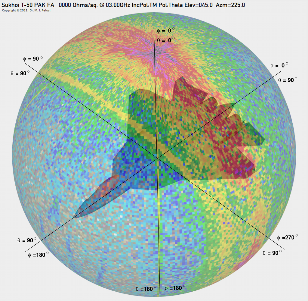


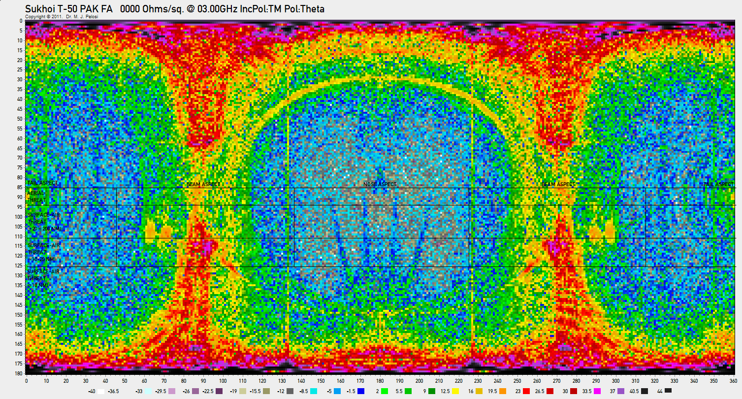

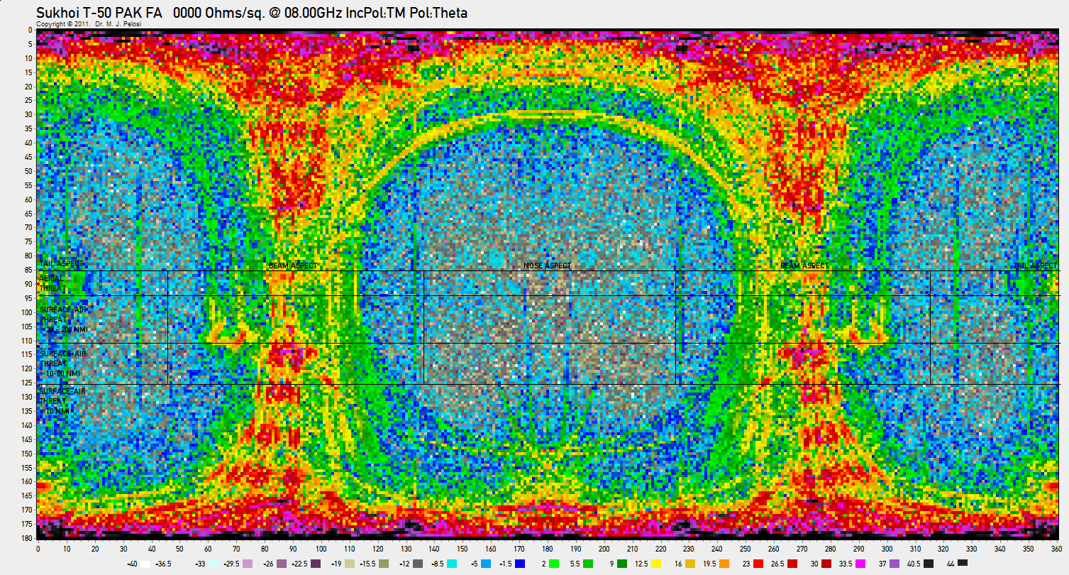
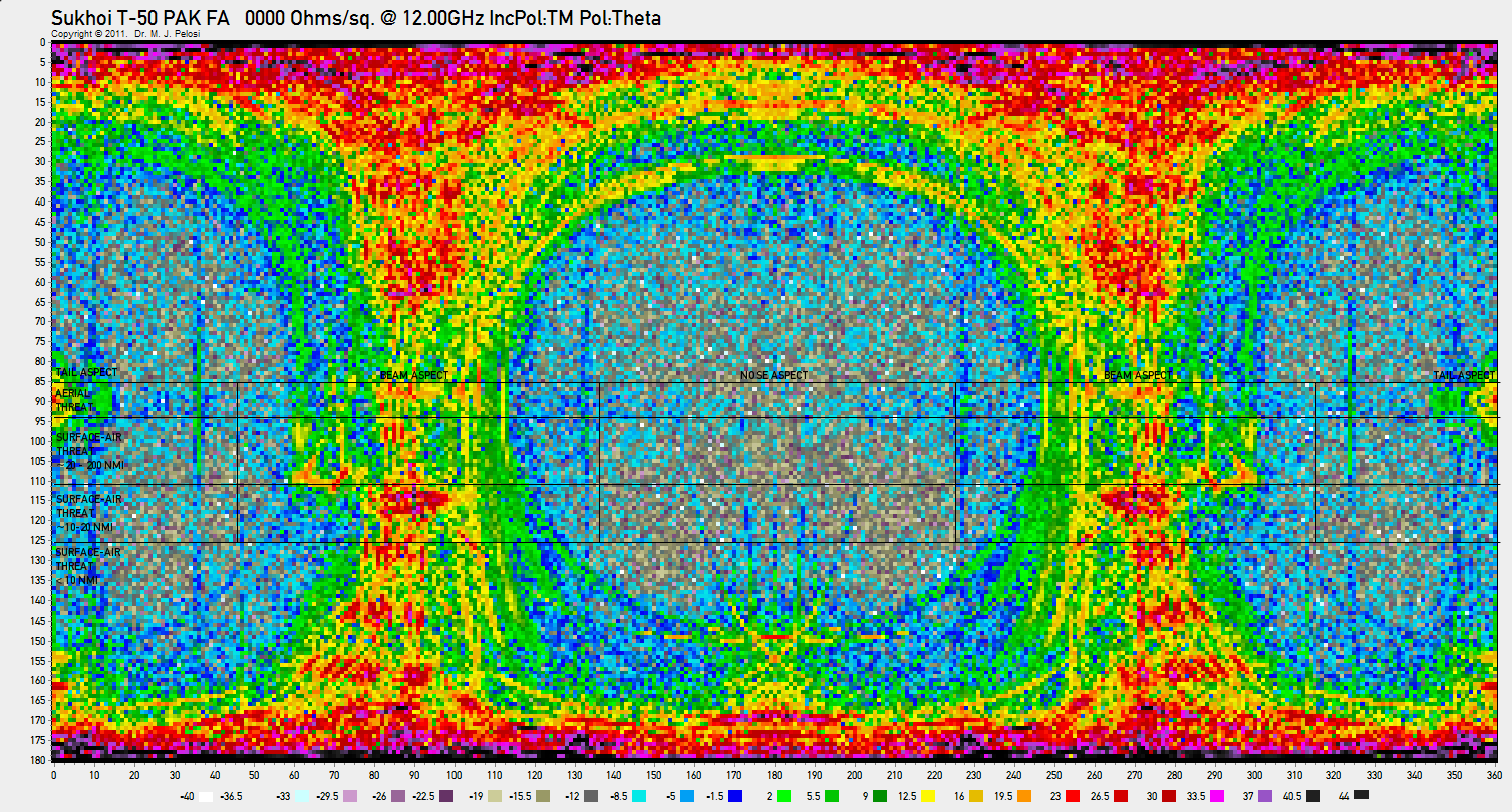
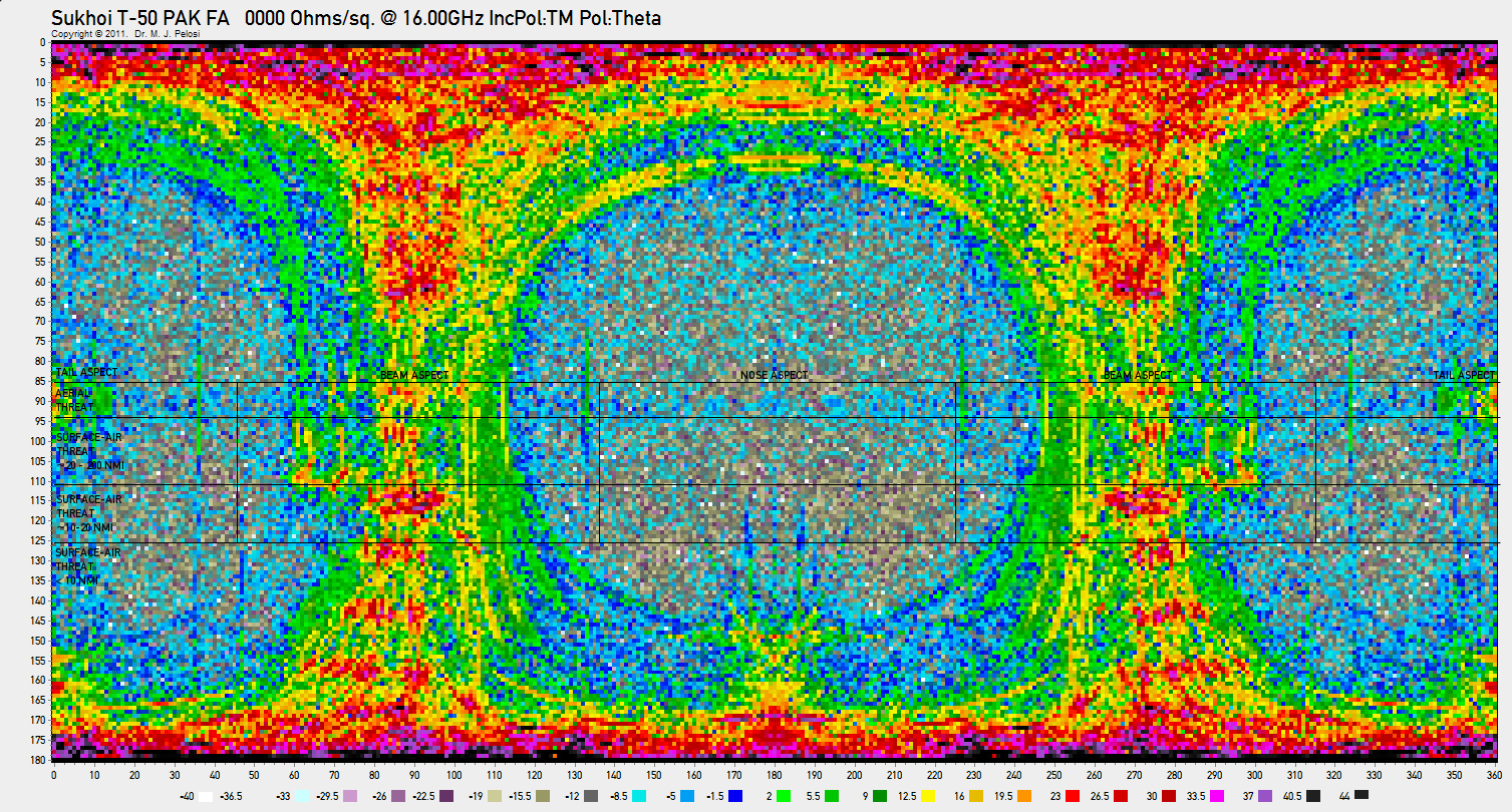

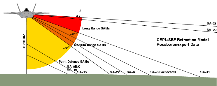
Table 3.
T-50 Specular RCS Model
Results With RAM
[V-Pol]
[Click Thumbnail to Enlarge] |
||||||||||
| Frequency |
150 MHz |
600 MHz |
1.2 GHz |
3.0 GHz |
6.0 GHz |
8.0 GHz |
12.0 GHZ |
16.0 GHz |
28.0 GHz |
|
| θ | Φ | 377 Ohm/sq Skin Coating / PEC Substrate |
||||||||
| 0 | 0 | ![Sukhoi-T-50-PAK-FA.mdb-00.15GHz-Rs0377-IncPol-TM-Pol-Theta-[E=000.0-A=000.0]](Rus-VLO/Sukhoi-T-50-PAK-FA.mdb-00.15GHz-Rs0377-IncPol-TM-Pol-Theta-%5BE=000.0-A=000.0%5D.png "Sukhoi-T-50-PAK-FA.mdb-00.15GHz-Rs0377-IncPol-TM-Pol-Theta-[E=000.0-A=000.0]") |
![Sukhoi-T-50-PAK-FA.mdb-00.60GHz-Rs0377-IncPol-TM-Pol-Theta-[E=000.0-A=000.0]](Rus-VLO/Sukhoi-T-50-PAK-FA.mdb-00.60GHz-Rs0377-IncPol-TM-Pol-Theta-%5BE=000.0-A=000.0%5D.png "Sukhoi-T-50-PAK-FA.mdb-00.60GHz-Rs0377-IncPol-TM-Pol-Theta-[E=000.0-A=000.0]") |
![Sukhoi-T-50-PAK-FA.mdb-01.20GHz-Rs0377-IncPol-TM-Pol-Theta-[E=000.0-A=000.0]](Rus-VLO/Sukhoi-T-50-PAK-FA.mdb-01.20GHz-Rs0377-IncPol-TM-Pol-Theta-%5BE=000.0-A=000.0%5D.png "Sukhoi-T-50-PAK-FA.mdb-01.20GHz-Rs0377-IncPol-TM-Pol-Theta-[E=000.0-A=000.0]") |
![Sukhoi-T-50-PAK-FA.mdb-03.00GHz-Rs0377-IncPol-TM-Pol-Theta-[E=000.0-A=000.0]](Rus-VLO/Sukhoi-T-50-PAK-FA.mdb-03.00GHz-Rs0377-IncPol-TM-Pol-Theta-%5BE=000.0-A=000.0%5D.png "Sukhoi-T-50-PAK-FA.mdb-03.00GHz-Rs0377-IncPol-TM-Pol-Theta-[E=000.0-A=000.0]") |
![Sukhoi-T-50-PAK-FA.mdb-06.00GHz-Rs0377-IncPol-TM-Pol-Theta-[E=000.0-A=000.0]](Rus-VLO/Sukhoi-T-50-PAK-FA.mdb-06.00GHz-Rs0377-IncPol-TM-Pol-Theta-%5BE=000.0-A=000.0%5D.png "Sukhoi-T-50-PAK-FA.mdb-06.00GHz-Rs0377-IncPol-TM-Pol-Theta-[E=000.0-A=000.0]") |
![Sukhoi-T-50-PAK-FA.mdb-08.00GHz-Rs0377-IncPol-TM-Pol-Theta-[E=000.0-A=000.0]](Rus-VLO/Sukhoi-T-50-PAK-FA.mdb-08.00GHz-Rs0377-IncPol-TM-Pol-Theta-%5BE=000.0-A=000.0%5D.png "Sukhoi-T-50-PAK-FA.mdb-08.00GHz-Rs0377-IncPol-TM-Pol-Theta-[E=000.0-A=000.0]") |
![Sukhoi-T-50-PAK-FA.mdb-12.00GHz-Rs0377-IncPol-TM-Pol-Theta-[E=000.0-A=000.0]](Rus-VLO/Sukhoi-T-50-PAK-FA.mdb-12.00GHz-Rs0377-IncPol-TM-Pol-Theta-%5BE=000.0-A=000.0%5D.png "Sukhoi-T-50-PAK-FA.mdb-12.00GHz-Rs0377-IncPol-TM-Pol-Theta-[E=000.0-A=000.0]") |
![Sukhoi-T-50-PAK-FA.mdb-16.00GHz-Rs0377-IncPol-TM-Pol-Theta-[E=000.0-A=000.0]](Rus-VLO/Sukhoi-T-50-PAK-FA.mdb-16.00GHz-Rs0377-IncPol-TM-Pol-Theta-%5BE=000.0-A=000.0%5D.png "Sukhoi-T-50-PAK-FA.mdb-16.00GHz-Rs0377-IncPol-TM-Pol-Theta-[E=000.0-A=000.0]") |
![Sukhoi-T-50-PAK-FA.mdb-28.00GHz-Rs0377-IncPol-TM-Pol-Theta-[E=000.0-A=000.0]](Rus-VLO/Sukhoi-T-50-PAK-FA.mdb-28.00GHz-Rs0377-IncPol-TM-Pol-Theta-%5BE=000.0-A=000.0%5D.png "Sukhoi-T-50-PAK-FA.mdb-28.00GHz-Rs0377-IncPol-TM-Pol-Theta-[E=000.0-A=000.0]") |
| 180 | 180 | ![Sukhoi-T-50-PAK-FA.mdb-00.15GHz-Rs0377-IncPol-TM-Pol-Theta-[E=180.0-A=180.0]](Rus-VLO/Sukhoi-T-50-PAK-FA.mdb-00.15GHz-Rs0377-IncPol-TM-Pol-Theta-%5BE=180.0-A=180.0%5D.png "Sukhoi-T-50-PAK-FA.mdb-00.15GHz-Rs0377-IncPol-TM-Pol-Theta-[E=180.0-A=180.0]") |
![Sukhoi-T-50-PAK-FA.mdb-00.60GHz-Rs0377-IncPol-TM-Pol-Theta-[E=180.0-A=180.0]](Rus-VLO/Sukhoi-T-50-PAK-FA.mdb-00.60GHz-Rs0377-IncPol-TM-Pol-Theta-%5BE=180.0-A=180.0%5D.png "Sukhoi-T-50-PAK-FA.mdb-00.60GHz-Rs0377-IncPol-TM-Pol-Theta-[E=180.0-A=180.0]") |
![Sukhoi-T-50-PAK-FA.mdb-01.20GHz-Rs0377-IncPol-TM-Pol-Theta-[E=180.0-A=180.0]](Rus-VLO/Sukhoi-T-50-PAK-FA.mdb-01.20GHz-Rs0377-IncPol-TM-Pol-Theta-%5BE=180.0-A=180.0%5D.png "Sukhoi-T-50-PAK-FA.mdb-01.20GHz-Rs0377-IncPol-TM-Pol-Theta-[E=180.0-A=180.0]") |
![Sukhoi-T-50-PAK-FA.mdb-03.00GHz-Rs0377-IncPol-TM-Pol-Theta-[E=180.0-A=180.0]](Rus-VLO/Sukhoi-T-50-PAK-FA.mdb-03.00GHz-Rs0377-IncPol-TM-Pol-Theta-%5BE=180.0-A=180.0%5D.png "Sukhoi-T-50-PAK-FA.mdb-03.00GHz-Rs0377-IncPol-TM-Pol-Theta-[E=180.0-A=180.0]") |
![Sukhoi-T-50-PAK-FA.mdb-06.00GHz-Rs0377-IncPol-TM-Pol-Theta-[E=180.0-A=180.0]](Rus-VLO/Sukhoi-T-50-PAK-FA.mdb-06.00GHz-Rs0377-IncPol-TM-Pol-Theta-%5BE=180.0-A=180.0%5D.png "Sukhoi-T-50-PAK-FA.mdb-06.00GHz-Rs0377-IncPol-TM-Pol-Theta-[E=180.0-A=180.0]") |
![Sukhoi-T-50-PAK-FA.mdb-08.00GHz-Rs0377-IncPol-TM-Pol-Theta-[E=180.0-A=180.0]](Rus-VLO/Sukhoi-T-50-PAK-FA.mdb-08.00GHz-Rs0377-IncPol-TM-Pol-Theta-%5BE=180.0-A=180.0%5D.png "Sukhoi-T-50-PAK-FA.mdb-08.00GHz-Rs0377-IncPol-TM-Pol-Theta-[E=180.0-A=180.0]") |
![Sukhoi-T-50-PAK-FA.mdb-12.00GHz-Rs0377-IncPol-TM-Pol-Theta-[E=180.0-A=180.0]](Rus-VLO/Sukhoi-T-50-PAK-FA.mdb-12.00GHz-Rs0377-IncPol-TM-Pol-Theta-%5BE=180.0-A=180.0%5D.png "Sukhoi-T-50-PAK-FA.mdb-12.00GHz-Rs0377-IncPol-TM-Pol-Theta-[E=180.0-A=180.0]") |
![Sukhoi-T-50-PAK-FA.mdb-16.00GHz-Rs0377-IncPol-TM-Pol-Theta-[E=180.0-A=180.0]](Rus-VLO/Sukhoi-T-50-PAK-FA.mdb-16.00GHz-Rs0377-IncPol-TM-Pol-Theta-%5BE=180.0-A=180.0%5D.png "Sukhoi-T-50-PAK-FA.mdb-16.00GHz-Rs0377-IncPol-TM-Pol-Theta-[E=180.0-A=180.0]") |
![Sukhoi-T-50-PAK-FA.mdb-28.00GHz-Rs0377-IncPol-TM-Pol-Theta-[E=180.0-A=180.0]](Rus-VLO/Sukhoi-T-50-PAK-FA.mdb-28.00GHz-Rs0377-IncPol-TM-Pol-Theta-%5BE=180.0-A=180.0%5D.png "Sukhoi-T-50-PAK-FA.mdb-28.00GHz-Rs0377-IncPol-TM-Pol-Theta-[E=180.0-A=180.0]") |
| 090 | 180 | ![Sukhoi-T-50-PAK-FA.mdb-00.15GHz-Rs0377-IncPol-TM-Pol-Theta-[E=090.0-A=180.0]](Rus-VLO/Sukhoi-T-50-PAK-FA.mdb-00.15GHz-Rs0377-IncPol-TM-Pol-Theta-%5BE=090.0-A=180.0%5D.png "Sukhoi-T-50-PAK-FA.mdb-00.15GHz-Rs0377-IncPol-TM-Pol-Theta-[E=090.0-A=180.0]") |
![Sukhoi-T-50-PAK-FA.mdb-00.60GHz-Rs0377-IncPol-TM-Pol-Theta-[E=090.0-A=180.0]](Rus-VLO/Sukhoi-T-50-PAK-FA.mdb-00.60GHz-Rs0377-IncPol-TM-Pol-Theta-%5BE=090.0-A=180.0%5D.png "Sukhoi-T-50-PAK-FA.mdb-00.60GHz-Rs0377-IncPol-TM-Pol-Theta-[E=090.0-A=180.0]") |
![Sukhoi-T-50-PAK-FA.mdb-01.20GHz-Rs0377-IncPol-TM-Pol-Theta-[E=090.0-A=180.0]](Rus-VLO/Sukhoi-T-50-PAK-FA.mdb-01.20GHz-Rs0377-IncPol-TM-Pol-Theta-%5BE=090.0-A=180.0%5D.png "Sukhoi-T-50-PAK-FA.mdb-01.20GHz-Rs0377-IncPol-TM-Pol-Theta-[E=090.0-A=180.0]") |
![Sukhoi-T-50-PAK-FA.mdb-03.00GHz-Rs0377-IncPol-TM-Pol-Theta-[E=090.0-A=180.0]](Rus-VLO/Sukhoi-T-50-PAK-FA.mdb-03.00GHz-Rs0377-IncPol-TM-Pol-Theta-%5BE=090.0-A=180.0%5D.png "Sukhoi-T-50-PAK-FA.mdb-03.00GHz-Rs0377-IncPol-TM-Pol-Theta-[E=090.0-A=180.0]") |
![Sukhoi-T-50-PAK-FA.mdb-06.00GHz-Rs0377-IncPol-TM-Pol-Theta-[E=090.0-A=180.0]](Rus-VLO/Sukhoi-T-50-PAK-FA.mdb-06.00GHz-Rs0377-IncPol-TM-Pol-Theta-%5BE=090.0-A=180.0%5D.png "Sukhoi-T-50-PAK-FA.mdb-06.00GHz-Rs0377-IncPol-TM-Pol-Theta-[E=090.0-A=180.0]") |
![Sukhoi-T-50-PAK-FA.mdb-08.00GHz-Rs0377-IncPol-TM-Pol-Theta-[E=090.0-A=180.0]](Rus-VLO/Sukhoi-T-50-PAK-FA.mdb-08.00GHz-Rs0377-IncPol-TM-Pol-Theta-%5BE=090.0-A=180.0%5D.png "Sukhoi-T-50-PAK-FA.mdb-08.00GHz-Rs0377-IncPol-TM-Pol-Theta-[E=090.0-A=180.0]") |
![Sukhoi-T-50-PAK-FA.mdb-12.00GHz-Rs0377-IncPol-TM-Pol-Theta-[E=090.0-A=180.0]](Rus-VLO/Sukhoi-T-50-PAK-FA.mdb-12.00GHz-Rs0377-IncPol-TM-Pol-Theta-%5BE=090.0-A=180.0%5D.png "Sukhoi-T-50-PAK-FA.mdb-12.00GHz-Rs0377-IncPol-TM-Pol-Theta-[E=090.0-A=180.0]") |
![Sukhoi-T-50-PAK-FA.mdb-16.00GHz-Rs0377-IncPol-TM-Pol-Theta-[E=090.0-A=180.0]](Rus-VLO/Sukhoi-T-50-PAK-FA.mdb-16.00GHz-Rs0377-IncPol-TM-Pol-Theta-%5BE=090.0-A=180.0%5D.png "Sukhoi-T-50-PAK-FA.mdb-16.00GHz-Rs0377-IncPol-TM-Pol-Theta-[E=090.0-A=180.0]") |
![Sukhoi-T-50-PAK-FA.mdb-28.00GHz-Rs0377-IncPol-TM-Pol-Theta-[E=090.0-A=180.0]](Rus-VLO/Sukhoi-T-50-PAK-FA.mdb-28.00GHz-Rs0377-IncPol-TM-Pol-Theta-%5BE=090.0-A=180.0%5D.png "Sukhoi-T-50-PAK-FA.mdb-28.00GHz-Rs0377-IncPol-TM-Pol-Theta-[E=090.0-A=180.0]") |
| 090 | 0 | ![Sukhoi-T-50-PAK-FA.mdb-00.15GHz-Rs0377-IncPol-TM-Pol-Theta-[E=090.0-A=000.0]](Rus-VLO/Sukhoi-T-50-PAK-FA.mdb-00.15GHz-Rs0377-IncPol-TM-Pol-Theta-%5BE=090.0-A=000.0%5D.png "Sukhoi-T-50-PAK-FA.mdb-00.15GHz-Rs0377-IncPol-TM-Pol-Theta-[E=090.0-A=000.0]") |
![Sukhoi-T-50-PAK-FA.mdb-00.60GHz-Rs0377-IncPol-TM-Pol-Theta-[E=090.0-A=000.0]](Rus-VLO/Sukhoi-T-50-PAK-FA.mdb-00.60GHz-Rs0377-IncPol-TM-Pol-Theta-%5BE=090.0-A=000.0%5D.png "Sukhoi-T-50-PAK-FA.mdb-00.60GHz-Rs0377-IncPol-TM-Pol-Theta-[E=090.0-A=000.0]") |
![Sukhoi-T-50-PAK-FA.mdb-01.20GHz-Rs0377-IncPol-TM-Pol-Theta-[E=090.0-A=000.0]](Rus-VLO/Sukhoi-T-50-PAK-FA.mdb-01.20GHz-Rs0377-IncPol-TM-Pol-Theta-%5BE=090.0-A=000.0%5D.png "Sukhoi-T-50-PAK-FA.mdb-01.20GHz-Rs0377-IncPol-TM-Pol-Theta-[E=090.0-A=000.0]") |
![Sukhoi-T-50-PAK-FA.mdb-03.00GHz-Rs0377-IncPol-TM-Pol-Theta-[E=090.0-A=000.0]](Rus-VLO/Sukhoi-T-50-PAK-FA.mdb-03.00GHz-Rs0377-IncPol-TM-Pol-Theta-%5BE=090.0-A=000.0%5D.png "Sukhoi-T-50-PAK-FA.mdb-03.00GHz-Rs0377-IncPol-TM-Pol-Theta-[E=090.0-A=000.0]") |
![Sukhoi-T-50-PAK-FA.mdb-06.00GHz-Rs0377-IncPol-TM-Pol-Theta-[E=090.0-A=000.0]](Rus-VLO/Sukhoi-T-50-PAK-FA.mdb-06.00GHz-Rs0377-IncPol-TM-Pol-Theta-%5BE=090.0-A=000.0%5D.png "Sukhoi-T-50-PAK-FA.mdb-06.00GHz-Rs0377-IncPol-TM-Pol-Theta-[E=090.0-A=000.0]") |
![Sukhoi-T-50-PAK-FA.mdb-08.00GHz-Rs0377-IncPol-TM-Pol-Theta-[E=090.0-A=000.0]](Rus-VLO/Sukhoi-T-50-PAK-FA.mdb-08.00GHz-Rs0377-IncPol-TM-Pol-Theta-%5BE=090.0-A=000.0%5D.png "Sukhoi-T-50-PAK-FA.mdb-08.00GHz-Rs0377-IncPol-TM-Pol-Theta-[E=090.0-A=000.0]") |
![Sukhoi-T-50-PAK-FA.mdb-12.00GHz-Rs0377-IncPol-TM-Pol-Theta-[E=090.0-A=000.0]](Rus-VLO/Sukhoi-T-50-PAK-FA.mdb-12.00GHz-Rs0377-IncPol-TM-Pol-Theta-%5BE=090.0-A=000.0%5D.png "Sukhoi-T-50-PAK-FA.mdb-12.00GHz-Rs0377-IncPol-TM-Pol-Theta-[E=090.0-A=000.0]") |
![Sukhoi-T-50-PAK-FA.mdb-16.00GHz-Rs0377-IncPol-TM-Pol-Theta-[E=090.0-A=000.0]](Rus-VLO/Sukhoi-T-50-PAK-FA.mdb-16.00GHz-Rs0377-IncPol-TM-Pol-Theta-%5BE=090.0-A=000.0%5D.png "Sukhoi-T-50-PAK-FA.mdb-16.00GHz-Rs0377-IncPol-TM-Pol-Theta-[E=090.0-A=000.0]") |
![Sukhoi-T-50-PAK-FA.mdb-28.00GHz-Rs0377-IncPol-TM-Pol-Theta-[E=090.0-A=000.0]](Rus-VLO/Sukhoi-T-50-PAK-FA.mdb-28.00GHz-Rs0377-IncPol-TM-Pol-Theta-%5BE=090.0-A=000.0%5D.png "Sukhoi-T-50-PAK-FA.mdb-28.00GHz-Rs0377-IncPol-TM-Pol-Theta-[E=090.0-A=000.0]") |
| 090 | 270 | ![Sukhoi-T-50-PAK-FA.mdb-00.15GHz-Rs0377-IncPol-TM-Pol-Theta-[E=090.0-A=270.0]](Rus-VLO/Sukhoi-T-50-PAK-FA.mdb-00.15GHz-Rs0377-IncPol-TM-Pol-Theta-%5BE=090.0-A=270.0%5D.png "Sukhoi-T-50-PAK-FA.mdb-00.15GHz-Rs0377-IncPol-TM-Pol-Theta-[E=090.0-A=270.0]") |
![Sukhoi-T-50-PAK-FA.mdb-00.60GHz-Rs0377-IncPol-TM-Pol-Theta-[E=090.0-A=270.0]](Rus-VLO/Sukhoi-T-50-PAK-FA.mdb-00.60GHz-Rs0377-IncPol-TM-Pol-Theta-%5BE=090.0-A=270.0%5D.png "Sukhoi-T-50-PAK-FA.mdb-00.60GHz-Rs0377-IncPol-TM-Pol-Theta-[E=090.0-A=270.0]") |
![Sukhoi-T-50-PAK-FA.mdb-01.20GHz-Rs0377-IncPol-TM-Pol-Theta-[E=090.0-A=270.0]](Rus-VLO/Sukhoi-T-50-PAK-FA.mdb-01.20GHz-Rs0377-IncPol-TM-Pol-Theta-%5BE=090.0-A=270.0%5D.png "Sukhoi-T-50-PAK-FA.mdb-01.20GHz-Rs0377-IncPol-TM-Pol-Theta-[E=090.0-A=270.0]") |
![Sukhoi-T-50-PAK-FA.mdb-03.00GHz-Rs0377-IncPol-TM-Pol-Theta-[E=090.0-A=270.0]](Rus-VLO/Sukhoi-T-50-PAK-FA.mdb-03.00GHz-Rs0377-IncPol-TM-Pol-Theta-%5BE=090.0-A=270.0%5D.png "Sukhoi-T-50-PAK-FA.mdb-03.00GHz-Rs0377-IncPol-TM-Pol-Theta-[E=090.0-A=270.0]") |
![Sukhoi-T-50-PAK-FA.mdb-06.00GHz-Rs0377-IncPol-TM-Pol-Theta-[E=090.0-A=270.0]](Rus-VLO/Sukhoi-T-50-PAK-FA.mdb-06.00GHz-Rs0377-IncPol-TM-Pol-Theta-%5BE=090.0-A=270.0%5D.png "Sukhoi-T-50-PAK-FA.mdb-06.00GHz-Rs0377-IncPol-TM-Pol-Theta-[E=090.0-A=270.0]") |
![Sukhoi-T-50-PAK-FA.mdb-08.00GHz-Rs0377-IncPol-TM-Pol-Theta-[E=090.0-A=270.0]](Rus-VLO/Sukhoi-T-50-PAK-FA.mdb-08.00GHz-Rs0377-IncPol-TM-Pol-Theta-%5BE=090.0-A=270.0%5D.png "Sukhoi-T-50-PAK-FA.mdb-08.00GHz-Rs0377-IncPol-TM-Pol-Theta-[E=090.0-A=270.0]") |
![Sukhoi-T-50-PAK-FA.mdb-12.00GHz-Rs0377-IncPol-TM-Pol-Theta-[E=090.0-A=270.0]](Rus-VLO/Sukhoi-T-50-PAK-FA.mdb-12.00GHz-Rs0377-IncPol-TM-Pol-Theta-%5BE=090.0-A=270.0%5D.png "Sukhoi-T-50-PAK-FA.mdb-12.00GHz-Rs0377-IncPol-TM-Pol-Theta-[E=090.0-A=270.0]") |
![Sukhoi-T-50-PAK-FA.mdb-16.00GHz-Rs0377-IncPol-TM-Pol-Theta-[E=090.0-A=270.0]](Rus-VLO/Sukhoi-T-50-PAK-FA.mdb-16.00GHz-Rs0377-IncPol-TM-Pol-Theta-%5BE=090.0-A=270.0%5D.png "Sukhoi-T-50-PAK-FA.mdb-16.00GHz-Rs0377-IncPol-TM-Pol-Theta-[E=090.0-A=270.0]") |
![Sukhoi-T-50-PAK-FA.mdb-28.00GHz-Rs0377-IncPol-TM-Pol-Theta-[E=090.0-A=270.0]](Rus-VLO/Sukhoi-T-50-PAK-FA.mdb-28.00GHz-Rs0377-IncPol-TM-Pol-Theta-%5BE=090.0-A=270.0%5D.png "Sukhoi-T-50-PAK-FA.mdb-28.00GHz-Rs0377-IncPol-TM-Pol-Theta-[E=090.0-A=270.0]") |
| 045 | 225 | ![Sukhoi-T-50-PAK-FA.mdb-00.15GHz-Rs0377-IncPol-TM-Pol-Theta-[E=045.0-A=225.0]](Rus-VLO/Sukhoi-T-50-PAK-FA.mdb-00.15GHz-Rs0377-IncPol-TM-Pol-Theta-%5BE=045.0-A=225.0%5D.png "Sukhoi-T-50-PAK-FA.mdb-00.15GHz-Rs0377-IncPol-TM-Pol-Theta-[E=045.0-A=225.0]") |
![Sukhoi-T-50-PAK-FA.mdb-00.60GHz-Rs0377-IncPol-TM-Pol-Theta-[E=045.0-A=225.0]](Rus-VLO/Sukhoi-T-50-PAK-FA.mdb-00.60GHz-Rs0377-IncPol-TM-Pol-Theta-%5BE=045.0-A=225.0%5D.png "Sukhoi-T-50-PAK-FA.mdb-00.60GHz-Rs0377-IncPol-TM-Pol-Theta-[E=045.0-A=225.0]") |
![Sukhoi-T-50-PAK-FA.mdb-01.20GHz-Rs0377-IncPol-TM-Pol-Theta-[E=045.0-A=225.0]](Rus-VLO/Sukhoi-T-50-PAK-FA.mdb-01.20GHz-Rs0377-IncPol-TM-Pol-Theta-%5BE=045.0-A=225.0%5D.png "Sukhoi-T-50-PAK-FA.mdb-01.20GHz-Rs0377-IncPol-TM-Pol-Theta-[E=045.0-A=225.0]") |
![Sukhoi-T-50-PAK-FA.mdb-03.00GHz-Rs0377-IncPol-TM-Pol-Theta-[E=045.0-A=225.0]](Rus-VLO/Sukhoi-T-50-PAK-FA.mdb-03.00GHz-Rs0377-IncPol-TM-Pol-Theta-%5BE=045.0-A=225.0%5D.png "Sukhoi-T-50-PAK-FA.mdb-03.00GHz-Rs0377-IncPol-TM-Pol-Theta-[E=045.0-A=225.0]") |
![Sukhoi-T-50-PAK-FA.mdb-06.00GHz-Rs0377-IncPol-TM-Pol-Theta-[E=045.0-A=225.0]](Rus-VLO/Sukhoi-T-50-PAK-FA.mdb-06.00GHz-Rs0377-IncPol-TM-Pol-Theta-%5BE=045.0-A=225.0%5D.png "Sukhoi-T-50-PAK-FA.mdb-06.00GHz-Rs0377-IncPol-TM-Pol-Theta-[E=045.0-A=225.0]") |
![Sukhoi-T-50-PAK-FA.mdb-08.00GHz-Rs0377-IncPol-TM-Pol-Theta-[E=045.0-A=225.0]](Rus-VLO/Sukhoi-T-50-PAK-FA.mdb-08.00GHz-Rs0377-IncPol-TM-Pol-Theta-%5BE=045.0-A=225.0%5D.png "Sukhoi-T-50-PAK-FA.mdb-08.00GHz-Rs0377-IncPol-TM-Pol-Theta-[E=045.0-A=225.0]") |
![Sukhoi-T-50-PAK-FA.mdb-12.00GHz-Rs0377-IncPol-TM-Pol-Theta-[E=045.0-A=225.0]](Rus-VLO/Sukhoi-T-50-PAK-FA.mdb-12.00GHz-Rs0377-IncPol-TM-Pol-Theta-%5BE=045.0-A=225.0%5D.png "Sukhoi-T-50-PAK-FA.mdb-12.00GHz-Rs0377-IncPol-TM-Pol-Theta-[E=045.0-A=225.0]") |
![Sukhoi-T-50-PAK-FA.mdb-16.00GHz-Rs0377-IncPol-TM-Pol-Theta-[E=045.0-A=225.0]](Rus-VLO/Sukhoi-T-50-PAK-FA.mdb-16.00GHz-Rs0377-IncPol-TM-Pol-Theta-%5BE=045.0-A=225.0%5D.png "Sukhoi-T-50-PAK-FA.mdb-16.00GHz-Rs0377-IncPol-TM-Pol-Theta-[E=045.0-A=225.0]") |
![Sukhoi-T-50-PAK-FA.mdb-28.00GHz-Rs0377-IncPol-TM-Pol-Theta-[E=045.0-A=225.0]](Rus-VLO/Sukhoi-T-50-PAK-FA.mdb-28.00GHz-Rs0377-IncPol-TM-Pol-Theta-%5BE=045.0-A=225.0%5D.png "Sukhoi-T-50-PAK-FA.mdb-28.00GHz-Rs0377-IncPol-TM-Pol-Theta-[E=045.0-A=225.0]") |
| 135 | 225 | ![Sukhoi-T-50-PAK-FA.mdb-00.15GHz-Rs0377-IncPol-TM-Pol-Theta-[E=135.0-A=225.0]](Rus-VLO/Sukhoi-T-50-PAK-FA.mdb-00.15GHz-Rs0377-IncPol-TM-Pol-Theta-%5BE=135.0-A=225.0%5D.png "Sukhoi-T-50-PAK-FA.mdb-00.15GHz-Rs0377-IncPol-TM-Pol-Theta-[E=135.0-A=225.0]") |
![Sukhoi-T-50-PAK-FA.mdb-00.60GHz-Rs0377-IncPol-TM-Pol-Theta-[E=135.0-A=225.0]](Rus-VLO/Sukhoi-T-50-PAK-FA.mdb-00.60GHz-Rs0377-IncPol-TM-Pol-Theta-%5BE=135.0-A=225.0%5D.png "Sukhoi-T-50-PAK-FA.mdb-00.60GHz-Rs0377-IncPol-TM-Pol-Theta-[E=135.0-A=225.0]") |
![Sukhoi-T-50-PAK-FA.mdb-01.20GHz-Rs0377-IncPol-TM-Pol-Theta-[E=135.0-A=225.0]](Rus-VLO/Sukhoi-T-50-PAK-FA.mdb-01.20GHz-Rs0377-IncPol-TM-Pol-Theta-%5BE=135.0-A=225.0%5D.png "Sukhoi-T-50-PAK-FA.mdb-01.20GHz-Rs0377-IncPol-TM-Pol-Theta-[E=135.0-A=225.0]") |
![Sukhoi-T-50-PAK-FA.mdb-03.00GHz-Rs0377-IncPol-TM-Pol-Theta-[E=135.0-A=225.0]](Rus-VLO/Sukhoi-T-50-PAK-FA.mdb-03.00GHz-Rs0377-IncPol-TM-Pol-Theta-%5BE=135.0-A=225.0%5D.png "Sukhoi-T-50-PAK-FA.mdb-03.00GHz-Rs0377-IncPol-TM-Pol-Theta-[E=135.0-A=225.0]") |
![Sukhoi-T-50-PAK-FA.mdb-06.00GHz-Rs0377-IncPol-TM-Pol-Theta-[E=135.0-A=225.0]](Rus-VLO/Sukhoi-T-50-PAK-FA.mdb-06.00GHz-Rs0377-IncPol-TM-Pol-Theta-%5BE=135.0-A=225.0%5D.png "Sukhoi-T-50-PAK-FA.mdb-06.00GHz-Rs0377-IncPol-TM-Pol-Theta-[E=135.0-A=225.0]") |
![Sukhoi-T-50-PAK-FA.mdb-08.00GHz-Rs0377-IncPol-TM-Pol-Theta-[E=135.0-A=225.0]](Rus-VLO/Sukhoi-T-50-PAK-FA.mdb-08.00GHz-Rs0377-IncPol-TM-Pol-Theta-%5BE=135.0-A=225.0%5D.png "Sukhoi-T-50-PAK-FA.mdb-08.00GHz-Rs0377-IncPol-TM-Pol-Theta-[E=135.0-A=225.0]") |
![Sukhoi-T-50-PAK-FA.mdb-12.00GHz-Rs0377-IncPol-TM-Pol-Theta-[E=135.0-A=225.0]](Rus-VLO/Sukhoi-T-50-PAK-FA.mdb-12.00GHz-Rs0377-IncPol-TM-Pol-Theta-%5BE=135.0-A=225.0%5D.png "Sukhoi-T-50-PAK-FA.mdb-12.00GHz-Rs0377-IncPol-TM-Pol-Theta-[E=135.0-A=225.0]") |
![Sukhoi-T-50-PAK-FA.mdb-16.00GHz-Rs0377-IncPol-TM-Pol-Theta-[E=135.0-A=225.0]](Rus-VLO/Sukhoi-T-50-PAK-FA.mdb-16.00GHz-Rs0377-IncPol-TM-Pol-Theta-%5BE=135.0-A=225.0%5D.png "Sukhoi-T-50-PAK-FA.mdb-16.00GHz-Rs0377-IncPol-TM-Pol-Theta-[E=135.0-A=225.0]") |
![Sukhoi-T-50-PAK-FA.mdb-28.00GHz-Rs0377-IncPol-TM-Pol-Theta-[E=135.0-A=225.0]](Rus-VLO/Sukhoi-T-50-PAK-FA.mdb-28.00GHz-Rs0377-IncPol-TM-Pol-Theta-%5BE=135.0-A=225.0%5D.png "Sukhoi-T-50-PAK-FA.mdb-28.00GHz-Rs0377-IncPol-TM-Pol-Theta-[E=135.0-A=225.0]") |
| 045 | 315 | ![Sukhoi-T-50-PAK-FA.mdb-00.15GHz-Rs0377-IncPol-TM-Pol-Theta-[E=045.0-A=315.0]](Rus-VLO/Sukhoi-T-50-PAK-FA.mdb-00.15GHz-Rs0377-IncPol-TM-Pol-Theta-%5BE=045.0-A=315.0%5D.png "Sukhoi-T-50-PAK-FA.mdb-00.15GHz-Rs0377-IncPol-TM-Pol-Theta-[E=045.0-A=315.0]") |
![Sukhoi-T-50-PAK-FA.mdb-00.60GHz-Rs0377-IncPol-TM-Pol-Theta-[E=045.0-A=315.0]](Rus-VLO/Sukhoi-T-50-PAK-FA.mdb-00.60GHz-Rs0377-IncPol-TM-Pol-Theta-%5BE=045.0-A=315.0%5D.png "Sukhoi-T-50-PAK-FA.mdb-00.60GHz-Rs0377-IncPol-TM-Pol-Theta-[E=045.0-A=315.0]") |
![Sukhoi-T-50-PAK-FA.mdb-01.20GHz-Rs0377-IncPol-TM-Pol-Theta-[E=045.0-A=315.0]](Rus-VLO/Sukhoi-T-50-PAK-FA.mdb-01.20GHz-Rs0377-IncPol-TM-Pol-Theta-%5BE=045.0-A=315.0%5D.png "Sukhoi-T-50-PAK-FA.mdb-01.20GHz-Rs0377-IncPol-TM-Pol-Theta-[E=045.0-A=315.0]") |
![Sukhoi-T-50-PAK-FA.mdb-03.00GHz-Rs0377-IncPol-TM-Pol-Theta-[E=045.0-A=315.0]](Rus-VLO/Sukhoi-T-50-PAK-FA.mdb-03.00GHz-Rs0377-IncPol-TM-Pol-Theta-%5BE=045.0-A=315.0%5D.png "Sukhoi-T-50-PAK-FA.mdb-03.00GHz-Rs0377-IncPol-TM-Pol-Theta-[E=045.0-A=315.0]") |
![Sukhoi-T-50-PAK-FA.mdb-06.00GHz-Rs0377-IncPol-TM-Pol-Theta-[E=045.0-A=315.0]](Rus-VLO/Sukhoi-T-50-PAK-FA.mdb-06.00GHz-Rs0377-IncPol-TM-Pol-Theta-%5BE=045.0-A=315.0%5D.png "Sukhoi-T-50-PAK-FA.mdb-06.00GHz-Rs0377-IncPol-TM-Pol-Theta-[E=045.0-A=315.0]") |
![Sukhoi-T-50-PAK-FA.mdb-08.00GHz-Rs0377-IncPol-TM-Pol-Theta-[E=045.0-A=315.0]](Rus-VLO/Sukhoi-T-50-PAK-FA.mdb-08.00GHz-Rs0377-IncPol-TM-Pol-Theta-%5BE=045.0-A=315.0%5D.png "Sukhoi-T-50-PAK-FA.mdb-08.00GHz-Rs0377-IncPol-TM-Pol-Theta-[E=045.0-A=315.0]") |
![Sukhoi-T-50-PAK-FA.mdb-12.00GHz-Rs0377-IncPol-TM-Pol-Theta-[E=045.0-A=315.0]](Rus-VLO/Sukhoi-T-50-PAK-FA.mdb-12.00GHz-Rs0377-IncPol-TM-Pol-Theta-%5BE=045.0-A=315.0%5D.png "Sukhoi-T-50-PAK-FA.mdb-12.00GHz-Rs0377-IncPol-TM-Pol-Theta-[E=045.0-A=315.0]") |
![Sukhoi-T-50-PAK-FA.mdb-16.00GHz-Rs0377-IncPol-TM-Pol-Theta-[E=045.0-A=315.0]](Rus-VLO/Sukhoi-T-50-PAK-FA.mdb-16.00GHz-Rs0377-IncPol-TM-Pol-Theta-%5BE=045.0-A=315.0%5D.png "Sukhoi-T-50-PAK-FA.mdb-16.00GHz-Rs0377-IncPol-TM-Pol-Theta-[E=045.0-A=315.0]") |
![Sukhoi-T-50-PAK-FA.mdb-28.00GHz-Rs0377-IncPol-TM-Pol-Theta-[E=045.0-A=315.0]](Rus-VLO/Sukhoi-T-50-PAK-FA.mdb-28.00GHz-Rs0377-IncPol-TM-Pol-Theta-%5BE=045.0-A=315.0%5D.png "Sukhoi-T-50-PAK-FA.mdb-28.00GHz-Rs0377-IncPol-TM-Pol-Theta-[E=045.0-A=315.0]") |
| 135 | 315 | ![Sukhoi-T-50-PAK-FA.mdb-00.15GHz-Rs0377-IncPol-TM-Pol-Theta-[E=135.0-A=315.0]](Rus-VLO/Sukhoi-T-50-PAK-FA.mdb-00.15GHz-Rs0377-IncPol-TM-Pol-Theta-%5BE=135.0-A=315.0%5D.png "Sukhoi-T-50-PAK-FA.mdb-00.15GHz-Rs0377-IncPol-TM-Pol-Theta-[E=135.0-A=315.0]") |
![Sukhoi-T-50-PAK-FA.mdb-00.60GHz-Rs0377-IncPol-TM-Pol-Theta-[E=135.0-A=315.0]](Rus-VLO/Sukhoi-T-50-PAK-FA.mdb-00.60GHz-Rs0377-IncPol-TM-Pol-Theta-%5BE=135.0-A=315.0%5D.png "Sukhoi-T-50-PAK-FA.mdb-00.60GHz-Rs0377-IncPol-TM-Pol-Theta-[E=135.0-A=315.0]") |
![Sukhoi-T-50-PAK-FA.mdb-01.20GHz-Rs0377-IncPol-TM-Pol-Theta-[E=135.0-A=315.0]](Rus-VLO/Sukhoi-T-50-PAK-FA.mdb-01.20GHz-Rs0377-IncPol-TM-Pol-Theta-%5BE=135.0-A=315.0%5D.png "Sukhoi-T-50-PAK-FA.mdb-01.20GHz-Rs0377-IncPol-TM-Pol-Theta-[E=135.0-A=315.0]") |
![Sukhoi-T-50-PAK-FA.mdb-03.00GHz-Rs0377-IncPol-TM-Pol-Theta-[E=135.0-A=315.0]](Rus-VLO/Sukhoi-T-50-PAK-FA.mdb-03.00GHz-Rs0377-IncPol-TM-Pol-Theta-%5BE=135.0-A=315.0%5D.png "Sukhoi-T-50-PAK-FA.mdb-03.00GHz-Rs0377-IncPol-TM-Pol-Theta-[E=135.0-A=315.0]") |
![Sukhoi-T-50-PAK-FA.mdb-06.00GHz-Rs0377-IncPol-TM-Pol-Theta-[E=135.0-A=315.0]](Rus-VLO/Sukhoi-T-50-PAK-FA.mdb-06.00GHz-Rs0377-IncPol-TM-Pol-Theta-%5BE=135.0-A=315.0%5D.png "Sukhoi-T-50-PAK-FA.mdb-06.00GHz-Rs0377-IncPol-TM-Pol-Theta-[E=135.0-A=315.0]") |
![Sukhoi-T-50-PAK-FA.mdb-08.00GHz-Rs0377-IncPol-TM-Pol-Theta-[E=135.0-A=315.0]](Rus-VLO/Sukhoi-T-50-PAK-FA.mdb-08.00GHz-Rs0377-IncPol-TM-Pol-Theta-%5BE=135.0-A=315.0%5D.png "Sukhoi-T-50-PAK-FA.mdb-08.00GHz-Rs0377-IncPol-TM-Pol-Theta-[E=135.0-A=315.0]") |
![Sukhoi-T-50-PAK-FA.mdb-12.00GHz-Rs0377-IncPol-TM-Pol-Theta-[E=135.0-A=315.0]](Rus-VLO/Sukhoi-T-50-PAK-FA.mdb-12.00GHz-Rs0377-IncPol-TM-Pol-Theta-%5BE=135.0-A=315.0%5D.png "Sukhoi-T-50-PAK-FA.mdb-12.00GHz-Rs0377-IncPol-TM-Pol-Theta-[E=135.0-A=315.0]") |
![Sukhoi-T-50-PAK-FA.mdb-16.00GHz-Rs0377-IncPol-TM-Pol-Theta-[E=135.0-A=315.0]](Rus-VLO/Sukhoi-T-50-PAK-FA.mdb-16.00GHz-Rs0377-IncPol-TM-Pol-Theta-%5BE=135.0-A=315.0%5D.png "Sukhoi-T-50-PAK-FA.mdb-16.00GHz-Rs0377-IncPol-TM-Pol-Theta-[E=135.0-A=315.0]") |
![Sukhoi-T-50-PAK-FA.mdb-28.00GHz-Rs0377-IncPol-TM-Pol-Theta-[E=135.0-A=315.0]](Rus-VLO/Sukhoi-T-50-PAK-FA.mdb-28.00GHz-Rs0377-IncPol-TM-Pol-Theta-%5BE=135.0-A=315.0%5D.png "Sukhoi-T-50-PAK-FA.mdb-28.00GHz-Rs0377-IncPol-TM-Pol-Theta-[E=135.0-A=315.0]") |
dBSM Scale |
||||||||||
 |
||||||||||
|
Table 4. T-50 Specular RCS Model Results With RAM [V-Pol] [Click Chart to Enlarge] |
|||||||||||||||||||||||||||
| 1.2 GHz | |||||||||||||||||||||||||||
![Chengdu_J-20_[2mm_Ferrite_-_4mm_CFC].mdb-01.20GHz-RsFromCoating-IncPol-TM-Pol-Theta](Rus-VLO/Sukhoi-T-50-PAK-FA.mdb-00.15GHz-Rs0377-IncPol-TM-Pol-Theta-E.png "Chengdu_J-20_[2mm_Ferrite_-_4mm_CFC].mdb-01.20GHz-RsFromCoating-IncPol-TM-Pol-Theta") |
|||||||||||||||||||||||||||
| 3.0 GHz | |||||||||||||||||||||||||||
 |
|||||||||||||||||||||||||||
| 6.0 GHz | |||||||||||||||||||||||||||
 |
|||||||||||||||||||||||||||
| 8.0 GHz | |||||||||||||||||||||||||||
 |
|||||||||||||||||||||||||||
| 12.0 GHZ | |||||||||||||||||||||||||||
 |
|||||||||||||||||||||||||||
| 16.0 GHz | |||||||||||||||||||||||||||
 |
|||||||||||||||||||||||||||
| 28.0 GHz | |||||||||||||||||||||||||||
 |
|||||||||||||||||||||||||||
|
|||||||||||||||||||||||||||
Conclusions
This study has explored the specular Radar Cross Section of the Sukhoi T-50 prototype aircraft shaping design. Simulations using a Physical Optics simulation algorithm were performed for frequencies of 150 MHz, 600 MHz, 1.2 GHz, 3.0 GHz, 6.0 GHz, 8.0 GHz, 12.0 GHz, 16.0 GHz and 28 GHz without an absorbent coating, and for frequencies of 1.2 GHz, 3.0 GHz, 6.0 GHz, 8.0 GHz, 12.0 GHz, 16.0 GHz with an absorbent coating, covering all angular aspects of the airframe.
If the production T-50 retains the axisymmetric nozzles and extant ventral fuselage design, the aircraft would still deliver robust Very Low Observable performance in the nose aspect angular sector, providing that effective RCS treatments are applied to suppress surface travelling waves, inlet and edge reflections.
If the production T-50 introduces a rectangular faceted nozzle design, and refinements to lower fuselage and side shaping, the design would present very good potential for good Very Low Observable performance in the S-band and above, for the nose and tail aspect angular sectors, with reasonable performance in the beam aspect angular sector. The extent to which this potential could be exploited would depend critically on the design of the nozzles and other shaping refinements.
In conclusion, this study has established through Physical Optics simulation across nine frequency bands, that no fundamental obstacles exist in the shaping design of the T-50 prototype, which might preclude its development into a genuine Very Low Observable design with constrained angular coverage.
Endnotes, References and Bibliography
1 Media Release, Компания "Сухой" приступила к летным испытаниям перспективного авиационного комплекса фронтовой авиации (ПАК ФА), OAO Sukhoi, 29th January, 2010.
2 Kopp, C. and Goon, P.A., Assessing the Sukhoi PAK-FA; Sukhoi/KnAAPO T-50/I-21/Article 701 PAK-FA; Перспективный Авиационный Комплекс Фронтовой Авиации, APA Analyses, Vol. VII, Issue 1, APA-2010-01, Feb 2010, URI: http://www.ausairpower.net/APA-2010-01.html.
3 Pelosi M.J. and Kopp C., A Preliminary Assessment of Specular Radar Cross Section Performance in the Chengdu J-20 Prototype, Air Power Australia Analyses, Vol VIII, Issue 3, APA-2011-03, Air Power Australia, Australia, pp. 1-35, Jul 2011, URI: http://www.ausairpower.net/APA-2011-03.html.
4 Knott, E.F., Schaeffer, J.F. and Tuley, M.T., Radar Cross Section, First Edition, Artech House, 1986; Knott, E.F., Schaeffer, J.F. and Tuley, M.T., Radar Cross Section, Second Edition, Artech House, 1993.
5 More recent quantitative RCS modelling of the J-20 axisymmetric nozzle design validates this observation in considerable detail. Please refer Kopp, C., Assessing Joint Strike Fighter Defence Penetration Capabilities, Air Power Australia Analyses, Vol.VI, Issue 1, APA-2009-01, 7th January 2009, URI: http://www.ausairpower.net/APA-2009-01.html, and Pelosi M.J. and Kopp C., A Preliminary Assessment of Specular Radar Cross Section Performance in the Chengdu J-20 Prototype, Air Power Australia Analyses, Vol VIII, Issue 3, APA-2011-03, Air Power Australia, Australia, pp. 1-35, Jul 2011, URI: http://www.ausairpower.net/APA-2011-03.html.
6 Chatzigeorgiadis, F., DEVELOPMENT OF CODE FOR A PHYSICAL OPTICS RADAR CROSS SECTION PREDICTION AND ANALYSIS APPLICATION, M.S. Thesis, NAVAL POSTGRADUATE SCHOOL, MONTEREY, CALIFORNIA, September 2004; Garrido, E.E. Jr, GRAPHICAL USER INTERFACE FOR A PHYSICAL OPTICS RADAR CROSS SECTION PREDICTION CODE, M.S. Thesis, NAVAL POSTGRADUATE SCHOOL, MONTEREY, CALIFORNIA, September 2000; Chatzigeorgiadis, F. and Jenn, D.C., “A MATLAB Physical Optics Prediction Code,” IEEE Antennas and Propagation Magazine, Vol. 46, No. 4, pp. 137-139, August 2004.
7 Kopp C., PolyChromatic Spherical Representation StL Format Generator Project Definition, August, 2011, Monash University, and Petroulias Z., Polychromatic Spherical Representation STL Format Generator, FIT1016 Final Report, Clayton School of Information Technology, Monash University, 11/16/2011.
8 Two publications detail a range of VHF radar types of interest, Fisher, R.D., Jr and Sweetman W., Too Little, Too Late, AirSea Battle concept may lag China’s capabilities, Defence Technology International, April, 2011 and Wise J.C., PLA Air Defence Radars, Technical Report APA-TR-2009-0103, Air Power Australia, January, 2009, URI: http://www.ausairpower.net/APA-PLA-IADS-Radars.html.
9 Yuzcelik, C.K, Radar Absorbing Material Design, M.S.Thesis, Naval Postgraduate School, Monterey, California, September, 2003.
Annex A Scales,
Bands,
Geometries
| dBSM |
30 |
20 |
10 |
0 |
-10 |
-20 |
-30 |
-40 |
-50 |
|||||
| m2 |
1,000.0 |
100.0 |
10.0 |
1.0 |
0.1 |
0.01 |
0.001 |
0.0001 |
0.00001 |
|||||
Table A.1 Conversion of RCS Values
[dBSM] vs [m2]
|
||||||||||||||

Figure A.3: Threat
depression
angles as a
function of type and missile kinematic range, for various contemporary
and legacy SAMs of Russian/Soviet manufacture (C. Kopp).
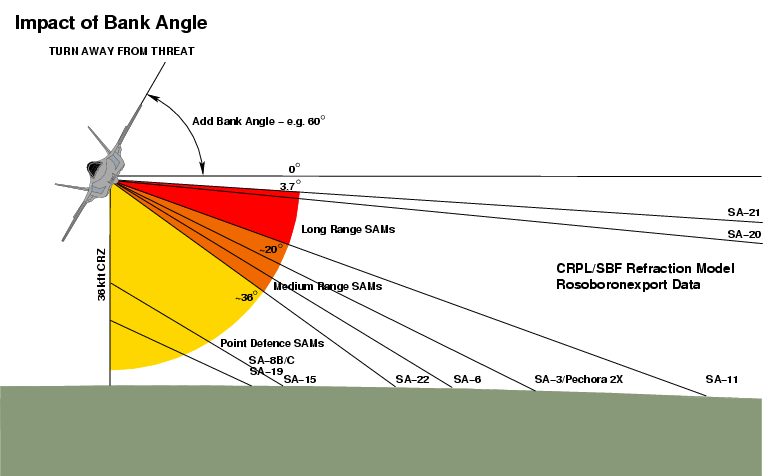
Figure A.4: The impact of bank angles on threat depression angles as a function of type and missile kinematic range, for various contemporary and legacy SAMs of Russian manufacture (C. Kopp).
Annex B Viewing RCS Plots
Radar Cross Section plots in this document are represented in two formats, PCSR and PCPR. Both were devised with the intention of providing an easily interpreted graphical representation which can display information with much greater density than the traditional polar plots of RCS.
The use of PCSR and PCPR thus permits a significantly greater volume of data to be presented, compared to polar plots, but with some loss of resolution in magnitude due to the coarse quantisation of the colour scale. This quantisation error is acceptable given the logarithmic scale for RCS magnitude employed.
As this document is published in HTML, it permits easy viewing at a number of resolutions, determined by the browser employed.
All PCSR and PCPR plots are set up with HTML links to the original plots, which are PNG files with respective resolutions of 1000 x 1000 pixels and 1507 x 810 pixels. Clicking on the plot will display it in a user's browser window, or in a separate tab.
Different browsers display PNG graphics differently. Some, like Firefox, Chrome or Safari will initially display the plot scaled to fit the window size. If the window size is smaller than the graphic, clicking on the graphic will enlarge it to its native size on the user display.
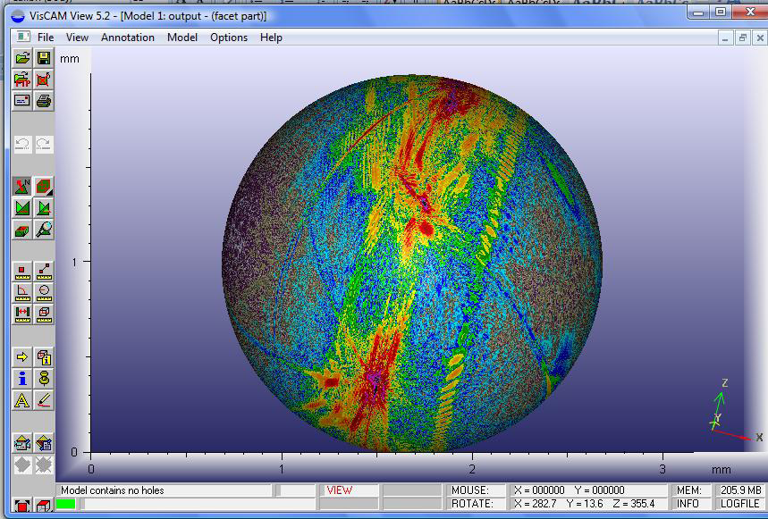
It was intended that detailed viewing of PCSR and PCPR plots be performed in the latter fashion, and text font sizes have been set accordingly. A portion of a PCPR plot at native resolution is below.
Annex C Glossary of Terms
- 2D TVC / Two Dimensional Thrust Vector Control: A
TVC arrangement which can control the direction of the engine thrust in
a
single geometrical plane, typically in the pitching axis.
- 3D TVC / Three Dimensional Thrust Vector Control: A TVC arrangement which can control the direction of the engine thrust in two mutually orthogonal geometrical planes.
- AESA: Active Electronically Steered [Scanned]
Array. A phased array antenna in which each element includes a solid
state
transmitter, receiver, and phase or delay beamsteering control
component.
- Azimuth Angles: The angle at which an illuminating
emitter is seen in the plane of flight of the aircraft, relative to
some datum such as the direction of flight.
- CoG / Centre of Gravity: The center of gravity is a
geometric property of any object. The center of gravity is the average
location of the weight of an object [NASA GRC].
- Carbon Nano-Tube (CNT): A CNT is one of eight
allotropes of carbon, where the molecule is formed as a single or
multiple walled tube, the walls of which are formed by connected
hexagonal rings; sometimes CNTs are termed buckytubes.
- CNT/Epoxy Absorbers: A RAM comprising an epoxy resin matrix loaded with Carbon Nanotube powder.
- dBSM: deciBels with reference to a square metre; a
logarithmic measure of RCS computed by multiplying the logarithm to the
base of ten of the RCS in square metres by ten.
- Depression Angle: The angle at which an illuminating emitter is seen below the plane of flight of the aircraft.
- DSI (Diverterless Supersonic Inlet): A DSI is an
inlet configuration where the inboard edge usually employed for
boundary layer control is replaced by a blister shaped protrusion; in
stealth design this is intended to remove the diffractive backscatter
from the inboard inlet leading edge.
- Elevation Angle: The angle at which an illuminating emitter is seen above the plane of flight of the aircraft.
- EO (Electro-Optical) Apertures: a cover usually
intended to protect an electro-optical sensor from the effects of its
physical environment without degrading its optical performance; the
optical mirror or lens system which focusses photons on to an optical
detection device such as an imaging chip.
- Ferrite/Epoxy Absorbers: A RAM comprising an epoxy resin matrix loaded with a ferrite powder.
- Gap Treatment: An absorber material or shaping
arrangement employed to reduce the RCS of a gap between two skin
panels, or a movable surface or door and fixed skin panel.
- Geometrical Diffraction: A method of computing RCS that is an extension of geometric optics that accounts for diffraction [Barton & Leonov].
- Lossy Surface Coating: A type of RAM which is
designed to produce electrical losses, but is not designed to
necessarily suppress specular reflections.
- Low Observable (LO): Early literature: any stealth aircraft; recent literature: a stealth aircraft with limited signature reduction, usually with an RCS between -10 and -30 dBSM.
- Matlab Language: An interpreted computer language
for mathematical expressions used by the Matlab code.
- NPS POFacets Code: A Physical Optics RCS simulator program designed and implemented at the Naval Postgraduate School in Monterey, California.
- Optics Scattering Regime: A scattering regime where the wavelength is smaller or very much smaller than the size of the object or shape scattering the wave.
- Panel Serration: A serration is a repetitive
triangular pattern used along an edge and intended to scatter surface
travelling waves in directions other than the normal to the line of the
edge.
- PCPR Format (PCPR): PolyChromatic Planar Representation (PCPR) is such a representation in which a rectangular area is divided into tiles by aspect angle pair {θ, Φ}. The colour of each tile represents the RCS from the angular direction determined by the path between the tile and the centroid of the aircraft.
- PCSR Format (PCSR): PolyChromatic Spherical Representation (PCSR) is such a representation in which a translucent sphere is rendered around a two-dimensional rendering of the aircraft, where the surface of the sphere is divided into tiles by aspect angle pair {θ, Φ}. The colour of each tile represents the RCS from the angular direction determined by the path between the tile and the centroid of the aircraft.
- Perfect Electrical Absorber (PEA): A material with a
characteristic impedance equal to that of free space and an infinite
loss for all wavelengths of interest.
- Perfect Electrical Conductor (PEC): A material with
a characteristic impedance of zero for all wavelengths of interest; an
idealised conductive metal.
- Physical Optics (PO): A method of computing RCS for
which the local current density at
each point on the illuminated portion of the body is assumed to be identical to the current density that would flow at that point on an infinite tangent plane [Barton & Leonov]. - Phased Array: “array antenna whose beam direction or radiation pattern is controlled primarily by the relative phases of the excitation coefficients of the radiating elements.” [Barton & Leonov].
- Radar Absorber: The term absorber refers to a radar absorbing structure or material (RAS or RAM), the purpose of which is to soak up incident energy and reduce the energy reflected back to the radar [Barton & Leonov].
- Radar Absorbent Materials (RAM): A material, such as
a coating, employed as a radar absorber.
- Radar Absorbent Structures (RAS): A structural component, such as a leading edge, employed as a radar absorber.
- Radar Cross Section (RCS): is “a measure of the reflective strength of a radar target.” The usual notation is σ. It is defined as σ = 4π Ps/Pi, where Ps is the power per unit solid angle scattered in a specific direction and Pi is the power per unit area in a plane wave incident on a scatterer from a specified direction [Barton & Leonov].
- Radome: A radome is “a cover usually intended to
protect an antenna from the effects of its physical environment without
degrading its electrical performance.” [Barton & Leonov].
- Raleigh Scattering Regime: A scattering regime where the wavelength is greater than the size of the object or shape scattering the wave; in Raleigh scattering, the backscatter is proportional to the inverse fourth power of the wavelength σ ∝ λ−4.
- Resonant Scattering Regime: A scattering regime where the wavelength is equal to or similar to the size of the object or shape scattering the wave.
- Specular RCS: RCS produced due to specular
scattering effects only.
- Specular Scattering: Scattering where a mirror-like reflection is produced by the scattering object or shape; usually the wavelength is smaller than the size of the object or shape scattering the wave.
- Thrust Vector Control (TVC): Any gas turbine or
rocket propulsion exhaust nozzle arrangement which permits the
direction of the exhaust efflux and thus thrust to be controlled.
Common arrangements include steerable nozzles, vanes or paddles.
- Very Low Observable (VLO): a stealth aircraft with very good signature reduction, usually with an RCS smaller than -30 dBSM.
Annex
D What the Simulation Does Not Demonstrate
- The PO simulator at this time does not model backscatter from edge diffraction effects, although the resulting error will be mitigated by the reality that in a mature production design these RCS contributions are reduced by edge treatments;
- The simulator at this time does not model backscatter from surface travelling wave effects. In the forward and aft hemispheres these can be dominant scattering sources where specular contributions are low. The magnitude of these RCS contributions is reduced by edge treatments, lossy surface coatings, gap treatments, and panel serrations;
- The simulator at this time does not model backscatter from the AESA bay in the passband of a bandpass radome, due to the absence of any data on the intended design of same, the resulting error will be mitigated by the reality that in a mature production design much effort will be expended in suppressing passband RCS contributions within the bay;
- The simulator at this time does not model backscatter from
in- and out-of-band impedance mismatches between the radomes and the
adjacent aircraft skin, and radomes are thus modelled as contiguous
surfaces of equal complex impedance to the adjacent skin panels. The
absence of data detailing the design of the bandpass radomes would
present a major challenge should such modelling be attempted, and could
be expected to degrade RCS performance results without necessarily
providing an accurate representation of the actual design;
- The simulator at this time does not model backscatter from the engine inlet tunnels or engine exhaust tailpipes, due to the absence of any data on the intended design of same. In the forward and aft hemispheres these can be dominant scattering sources where specular contributions are low. The magnitude of these RCS contributions is reduced by suppressing these RCS contributions with absorbers, and in the case of inlet tunnels, by introducing a serpentine geometry to increase the number of bounces;
- The simulator at this time does not model structural mode RCS contributions from antenna and EO apertures, panel joins, panel and door gaps, fasteners and other minor contributors; although the resulting error will be mitigated by the reality that in a mature production design these RCS contributions are reduced by RCS reduction treatments.
- The PO computational algorithm performs most accurately at broadside or near normal angles of incidence, with decreasing accuracy at increasingly shallow angles of incidence, reflecting the limitions of PO modelling. The simulator does not implement the Mitzner/Ufimtsev corrections for edge currents. While a number of test runs with basic shapes showed good agreement between the PO simulation and backscatter peaks in third party test sample measurements, even at incidence angles below 10°, characteristically PO will underestimate backscatter in nulls. This limitation must be considered when assessing results for the nose and tail aspects, where most specular RCS contributions arise at very shallow angles39.
- The PO computational algorithm performs best where the product of wave number and dimension ka ≥ 5, where k ≈ 2πf [Table 5.1 in (1)], yielding errors much less than 1 dB. Knott cites good agreement for cylinders as small as 1.5 wavelengths in diameter1.
- The simulator does not account for a number of environmental factors, such as air density profile at the aircraft skin boundary layer, thermal variations in absorbent material properties, and moisture precipitation. RCS contributions from these sources are negligible for the principal lobe magnitudes studied.
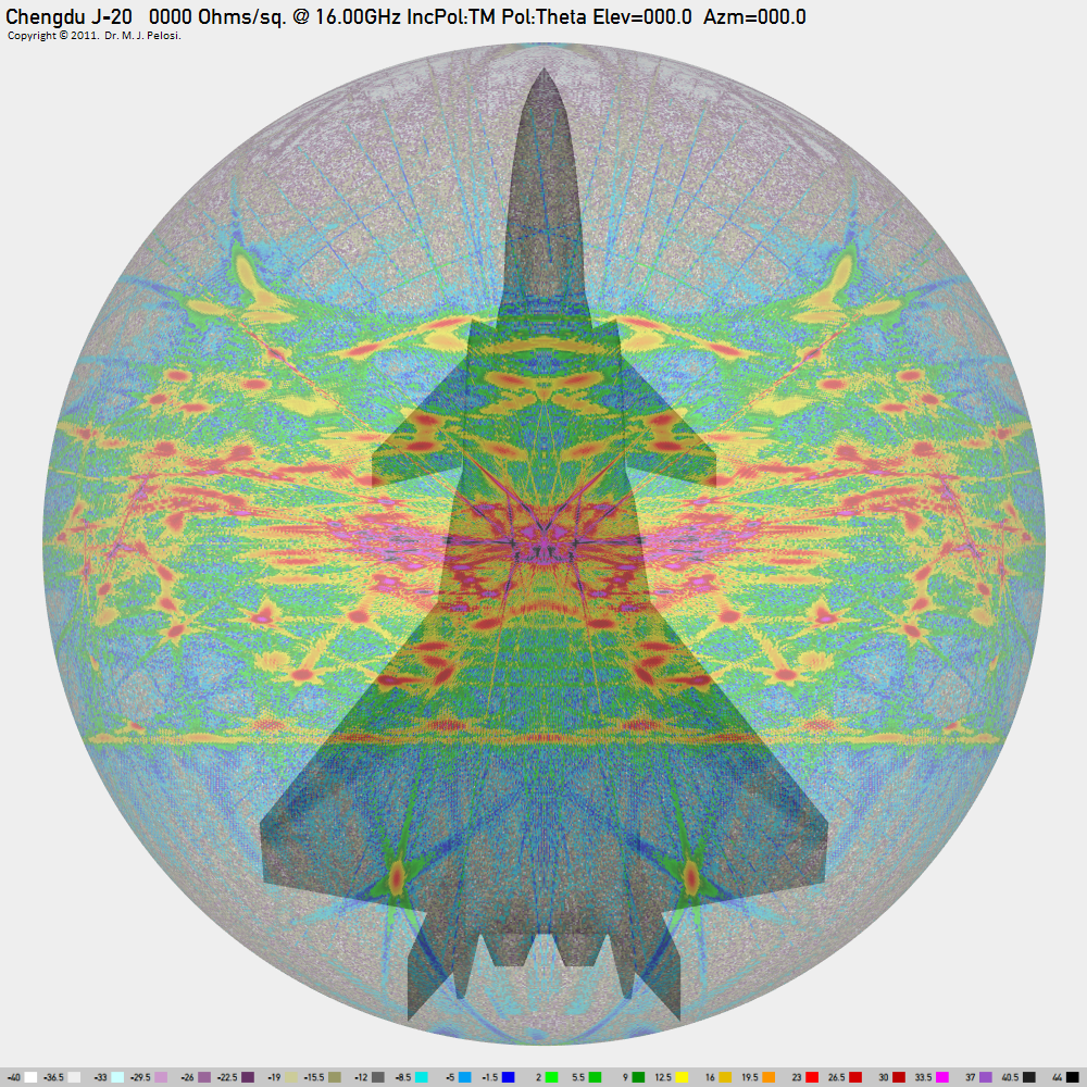
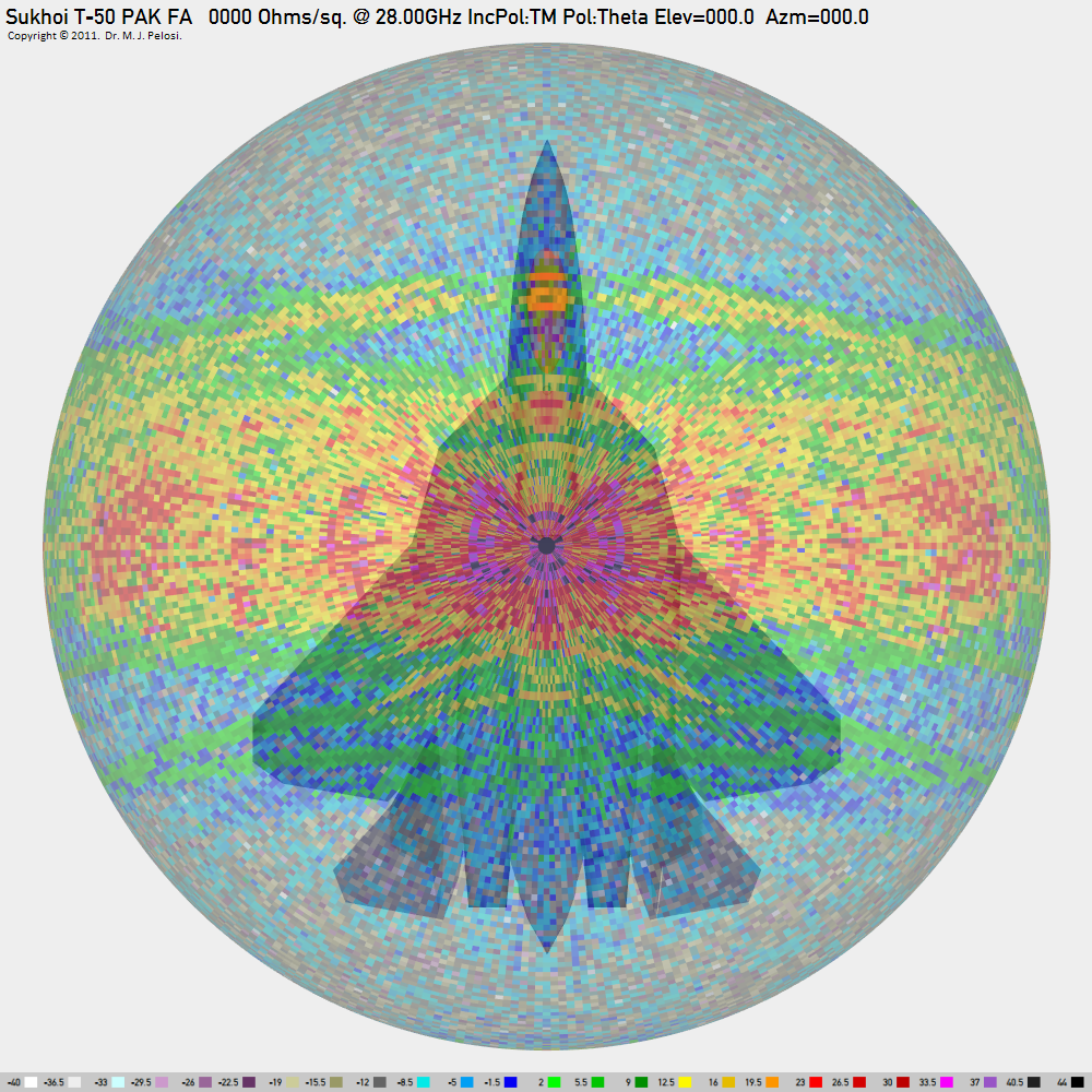
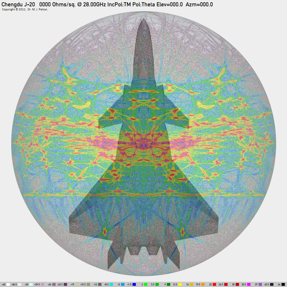
Annex E
Comparative
Analysis of
Specular RCS - T-50 Versus J-20
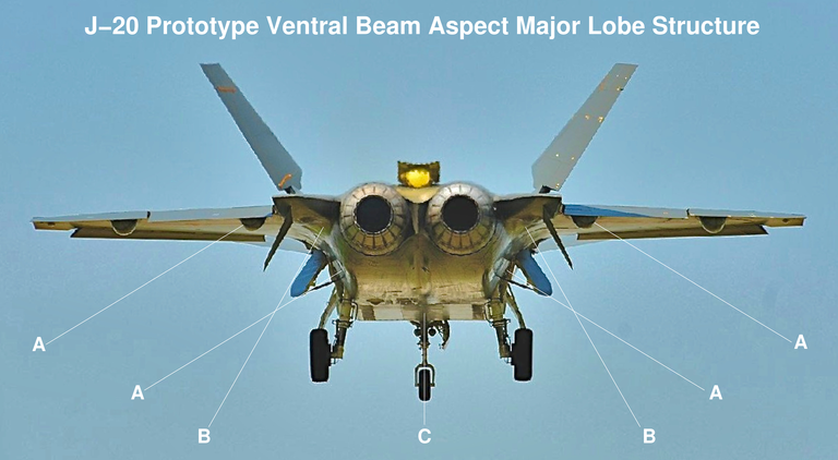
Figure E.1. The J-20 has two major
lobes in the left and
right beam aspect angular sectors, for convenience labelled A and B,
with the flat lower fuselage mainlobe labelled C (Chinese Internet
image).
| Table E.1. T-50/J-20 Specular
RCS Model Results With PEC [V-Pol] [Click Chart to Enlarge] |
|
| 150 MHz |
|
 |
 |
| 600 MHz | |
 |
 |
| 1.2 GHz | |
 |
 |
| 3.0 GHz | |
 |
 |
| 6.0 GHz | |
 |
 |
| 8.0 GHz | |
 |
 |
| 12.0 GHz | |
 |
 |
| 16.0 GHz | |
 |
 |
| 28.0 GHz | |
 |
 |
| dBSM Scale | |
|
|
Annex
F Additional Notes on Physical Optics RCS Modelling
All object model surfaces are approximated using triangular facets, which is especially convenient as this technique is also employed in commonly used vector graphic modelling schemes for CGI, such as the Stereo Lithographic (StL) format.
The PO method is inherently limited as it does not consider edge contributions, and accuracy suffers as the angle of incidence departs from the broadside or normal to a contributing facet. The latter makes the PO method suitable for identifying major specular contributors to vehicle RCS, but not minor contributors.
An abbreviated summary of the basic principles of the PO method, cited from Chatzigeorgiadis and Jenn follows6.
The backscatter behaviour produced by a triangular facet represents a special case of the backscatter behaviour produced by a body of an arbitrary shape. The expression for the scattered field produced by a triangular facet can thus be derived from the expression which can be obtained for an arbitrary body. Consider an arbitrary scattering body placed at the origin of the coordinate system, with the observation point placed at coordinates (x, y, z), refer Figure F.1.
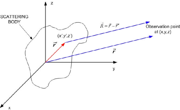
Figure F.1 Far Field Scattering from an Arbitrary Body (Jenn, 1995).
As we assume a far field geometry, the vectors r→ and R→ can be safely assumed to be parallel. If we assume the body has been divided into infinitesimally small volumes v' each at coordinates (x', y', z'), then the position vector to a point source is:
 |
EQ.1 |
The unit vector in the direction of the point of observation is:
 where u, v, w are defined as: |
EQ.2 |
 and where θ and Φ are
the angular components in the spherical coordinate system, for the
point of observation.
|
EQ.3 |
If we assume the magnetic volume current to be J→m = 0, the field scattered by the body can be found from EQ.4:
 Where: J→ is the volume current; Z0 is the intrinsic impedance of free space; k = 2π/λ or wave number; and g is defined to be: |
EQ.4 |
 |
EQ.5 |
The electric field has components only in the θ and Φ directions.
Now consider a triangular facet of arbitrary orientation in space, which is defined by three vertices, denoted 1, 2 and 3, in Figure F.2:
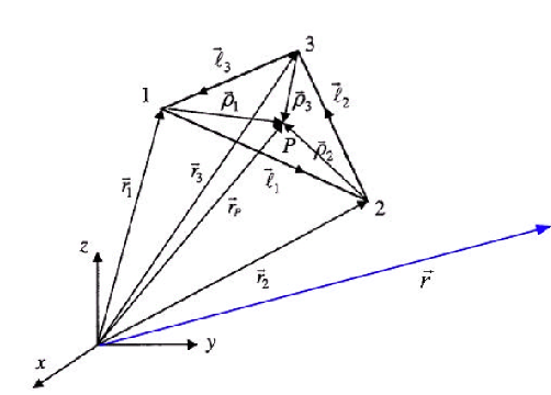
Figure F.2 Facet geometry and
orientation
(Jenn, 1995).
P is the integration point at (xp,
yp, zp), which corresponds to the coordinates
(x', y', z') for the integration point in the arbitrary body
previously discussed. We define its position vector as:
 |
EQ.6 |
 Where J→s is the surface current, A the facet area, dsp the differential surface area and g defined thus: |
EQ.7 |
 |
EQ.8 |
To perform this computation, we need explore the radiation integral for a triangular facet. Assume a triangular facet of arbitrary orientation, which has vertices in a cartesian coordinate system of (xn, yn, zn), for vertices 1, 2 and 3. Vertices are labelled counter-clockwise, or if following a right hand rule, where the thumb of the right hand points in the direction of the normal to the facet face. This is depicted in Figure F.3.
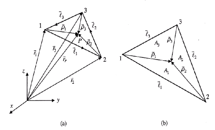
Figure F.3 Facet geometry
(Jenn, 1995).
Position vectors for each vertex are given as:
 |
EQ.9 |
 |
EQ.10 |
 |
EQ.11 |
 for which (ui, vi, wi) are the direction cosine; and R^ is the radial unit vector between the origin to the source located at angle (θi, Φi). |
EQ.12 |
 |
EQ.13 |
 |
EQ.14 |
 |
EQ.15 |
 |
EQ.16 |
 |
EQ.17 |
 |
EQ.18 |
 |
EQ.19 |
 |
EQ.20 |
 where h is defined thus: |
EQ.21 |
 |
EQ.22 |
 |
EQ.23 |
To compute the scattered field produced by the induced current in the facet, we substitute the simplified expression into the radiation integral in EQ.7. This yields:
 |
EQ.24 |
 |
EQ.25 |
A more detailed treatment is available in Chatzigeorgiadis and Jenn6.
Air Power Australia Analyses ISSN 1832-2433
|
|||||||||||||
|
|
|
|
|
|
|
|
||||||
|
|
|
|
|
|
|
|
||||||
 [Click for more ...]") |
|||||||||||||
| Artwork, graphic design, layout and text © 2004 - 2014 Carlo Kopp; Text © 2004 - 2014 Peter Goon; All rights reserved. Recommended browsers. Contact webmaster. Site navigation hints. Current hot topics. | |||||||||||||
|
Site Update
Status:
$Revision: 1.753 $
Site History: Notices
and
Updates / NLA Pandora Archive
|
|||||||||||||
|
|
Tweet | Follow @APA_Updates | |||||||||||
|
|
|||||||||||||
|
|
|||||||||||||